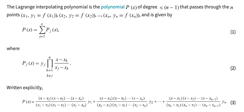
groth16 demystified

1. Introduction

Goldwasser, Micali and Rackoff [GMR89] introduced zero-knowledge proofs that enable a prover to convince a verifier that a statement is true without revealing anything else. They have three core properties:

  • Completeness: Given a statement and a witness, the prover can convince the verifier.
  • Soundness: A malicious prover cannot convince the verifier of a false statement.
  • Zero-knowledge: The proof does not reveal anything but the truth of the statement

1.1. Contribution

Succinct NIZK We construct a NIZK argument for arithmetic circuit satisfiability where a proof consists of only 3 group elements. In addition to being small, the proof is also easy to verify. The verifier just needs to compute a number of exponentiations proportional to the statement size and check a single pairing product equation, which only has 3 pairings.

2. Preliminaries

2.1 Bilinear Groups

We will work over bilinear groups \((p, \mathbb{G_{1}}, \mathbb{G_{2}}, \mathbb{G_{T}} , e, g, h)\) with the following properties:

  • \(\mathbb{G_{1}}, \mathbb{G_{2}}, \mathbb{G_{T}} \)are groups of prime order \(p\)
  • The pairing \( e:\mathbb{G_{1}} \times \mathbb{G_{2}} \rightarrow \mathbb{G_{T}}\) is a bilinear map
  • \(g\) is a generator for \(\mathbb{G_{1}}\), \(h\) is a generator for \(\mathbb{G_{2}}\), and \(e(g,h)\) is a generator for \(\mathbb{G_{T}}\)

There are many ways to set up bilinear groups both as symmetric bilinear groups where \(\mathbb{G_{1}} = \mathbb{G_{1}}\) and as asymmetric bilinear groups where \(\mathbb{G_{1}} \neq \mathbb{G_{1}}\). Galbraith, Paterson and Smart [GPS08] classify bilinear groups as Type I where \(\mathbb{G_{1}} = \mathbb{G_{2}}\), Type II where there is an efficiently computable non-trivial homomorphism \(\Phi : \mathbb{G_{2}} \rightarrow \mathbb{G_{1}}\), and Type III where no such efficiently computable homomorphism exists in either direction between \(\mathbb{G_{1}}\) and \(\mathbb{G_{2}}\). Type III bilinear groups are the most efficient type of bilinear groups and hence the most relevant for practical applications.
As a notation for group elements, we write \( \lbrack a \rbrack_{1} \) for \( g^a\), \( \lbrack b \rbrack_{2}\) for \( h^b\) and \( \lbrack c \rbrack_{T}\) for \(e(g,h)^{c} \). A vector of group elements will be represented as \( \lbrack \mathbf{a} \rbrack_{i} \). Given two vectors of \(n\) group elements \( \lbrack \mathbf{a} \rbrack_{1} \) and \( \lbrack \mathbf{b} \rbrack_{2} \), we define their dot product as \( \lbrack \mathbf{a} \rbrack_{1} \cdot \lbrack \mathbf{b} \rbrack_{2} = \lbrack \mathbf{a} \cdot \mathbf{b} \rbrack_{T} \), which can be efficiently computed using the pairing \(e\).

Protocol

R1CS

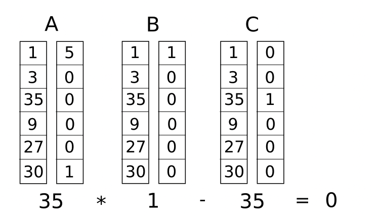
Let \(A, B,C\) be \(m \times n\) matrices with entries from field \( \mathbb{F}\). An R1CA instance takes the form:
\[ \tag{1} (z\cdot A) \odot (z \cdot B) = z \cdot C \]
where \(\cdot\) denotes dot product and \(\odot\) denotes entry-wise product. we required \(z_0 = 1\) because otherwise, \(z=0\) would satisfy every R1CS instance.

note: m is the number of witness, n is number of constraints.

QAP

Consider an arithmetic circuit \({C, x,y}\) with addition and multiplication gates, where we designate some input/output wires to specify statement \(x\) and the rest of the wires to specify witness \(\omega\). The prover wants to convince the verifier that there exists a witness \(\omega\) such that \(C(x,\omega) = y\). If the prover knows a witness \(\omega\), then they know a vector \(z\) that satisfies the constraint of the R1CS. We set the solution vector \(z\) to be an \(m\)-length vector, where \(z_0=1\). each remaining entry of \(z\) represents either the statement \(x\) or witness \(\omega\). Namely, \(x=\{z_1, …, z_l\}\) and \(\omega=\{ z_{l+1},…,z_{m}\}\).

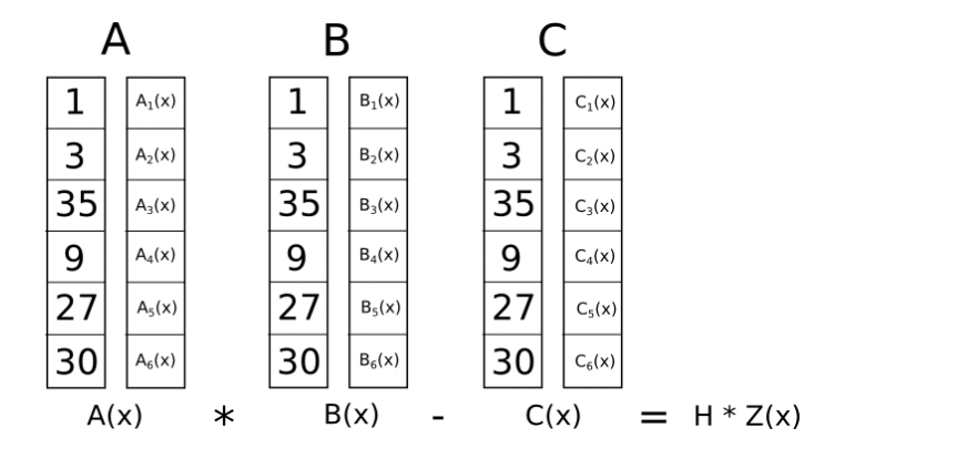
Choose arbitrary distinct elements \(\{r_1, r_2, …, r_n\} \in \mathbb{F}\), where \(r_i\) indicating gate number. We define polynomial coefficient matrices such that each polynomial evaluation encodes an R1CS constraint:
\[\tag{2} A_i(r_q) = A_{i,q} \quad B_i(r_q) = B_{i,q} \quad C_i(r_q) = C_{i,q} \]
where \(i = 1,…,m; q=1,…,n\)
we sum these polynomial vector groups to define three univariate polynomials
\[ \tag{3} A(X) = \sum_{i=0}^{m}z_iA_i(X) \quad B(X) = \sum_{i=0}^{m}z_iB_i(X) \quad C(X) = \sum_{i=0}^{m}z_iC_i(X)\]
The witness vector \(z\), where \(z_0=1\), will satisfy the \(n\) equations in the R1CS instance if and only if at each point \(\{r_1, r_2,…r_n\}\):
\[ \tag{4} \sum_{i=0}^{m}z_iA_i(r_q) \cdot \sum_{i=0}^{m}z_iB_i(r_q) = \sum_{i=0}^{m}z_iC_i(r_q)\]

We know \(t(x):=(x-r_1)(x-r_2)…(x-r_n) =\prod_{q=1}^{n}(x-r_q)\) is the lowest degree monomial such that \(t(r_q)=0\) in each point. Thus, we can reformulate the above as:

\[ \tag{5} \sum_{i=0}^{m}z_iA_i(r_q) \cdot \sum_{i=0}^{m}z_iB_i(r_q) = \sum_{i=0}^{m}z_iC_i(r_q) \mod t(X)\]
Thus, the derived QAP defines the following relation R, where \(z_0 =1\)
\(
\begin{equation}
R =
\begin{cases}
x=(z_1,…,z_l) \in \mathbb{F}^l \\
\omega =(z_{l+1},…,z_m) \in \mathbb{F}^{m-l} \\
\sum_{i=0}^{m}z_iA_i(r_q) \cdot \sum_{i=0}^{m}z_iB_i(r_q) = \sum_{i=0}^{m}z_iC_i(r_q) \mod t(X)
\end{cases}
\end{equation}
\)

Verifying the QAP

Let these QAP polynomials be defined as \(A(X), B(X), C(X)\) where \(A(X) = \sum_{i=0}^{m}z_iA_i(X)\) and similarly for \(B,C\). Let \(g_z\) denote the d-degree polynomial, where \(d\le 2(n-1)\) since \(A(X), B(X), C(X)\) are at most degree \(n-1\)
\[ g_z(X) = \sum_{i=0}^{m}z_iA_i(X) \cdot \sum_{i=0}^{m} z_iB_i(X) - \sum_{i=0}^{m}z_iC_i(X) \]
To verify the QAP, we show the existence of a low-degree polynomial \( h(X) = \frac{g_z(X)}{t(X)} \)

Non-Interactive Zero-Knowledge(NIZK) arguments for QAP

Consider \(R=(p, \mathbb{G_1}, \mathbb{G_2}, \mathbb{G_T}, e, g_1, g_2, l, \{A_i(X), B_i(X), C_i(X)\}, t(X))\)

Recall \(x=(z_1,…,z_l) \in \mathbb{Z}_{p}^{l}\)

and \(\omega=(z_{l+1},…,z_m) \in \mathbb{Z}_{p}^{m-l}\), where \(z_0=1\). The relation defines
\[ A(X) \cdot B(X) -C(X) = h(X)t(X) \]

Trusted Setup

Groth16 uses a two-step trusted setup to generate the common reference string (CRS). The trusted setup consists of two phases: the first is generic and the second is specific to the circuit.
As our CRS, we generate the random field elements \(\alpha, \beta, \gamma, \delta, \tau \in \mathbb{Z}_{p}^{*}\)

phase 1 powers of tau

\( (\lbrack \tau^0 \rbrack_{1}, \lbrack \tau^1 \rbrack_{1}, \lbrack \tau^2 \rbrack_{1},…, \lbrack \tau^{2(n-1)} \rbrack_{1}) \)
\( (\lbrack \tau^0 \rbrack_{2}, \lbrack \tau^1 \rbrack_{2}, \lbrack \tau^2 \rbrack_{2},…, \lbrack \tau^{n-1} \rbrack_{2}) \)
\( \lbrack \alpha \rbrack_{1} \cdot (\lbrack \tau^0 \rbrack_{1}, \lbrack \tau^1 \rbrack_{1}, \lbrack \tau^2 \rbrack_{1},…, \lbrack \tau^{n-1} \rbrack_{1}) \)
\( \lbrack \beta \rbrack_{1} \cdot (\lbrack \tau^0 \rbrack_{1}, \lbrack \tau^1 \rbrack_{1}, \lbrack \tau^2 \rbrack_{1},…, \lbrack \tau^{n-1} \rbrack_{1}) \)
\(\lbrack \beta \rbrack_{2}\)

phase 2

Given \(A_i, B_i, C_i\), we define polynomials \(L_i: L_i(X) = \beta \cdot A_i(X) + \alpha \cdot B_i(X) +C_i(X) \). We cannot compute \(L_i(X)\) directly because \(\alpha\) and \(\beta\) are private, so instead, we construct \(L_i(\tau)\cdot g_i\) using values computed in Phase 1.

providng key (pk)

\((\lbrack \alpha \rbrack_{1}, \lbrack \beta \rbrack_{1}, \lbrack \delta \rbrack_{1})\)
\((\lbrack \tau^0 \rbrack_{1}, \lbrack \tau^2 \rbrack_{1}, \lbrack \tau^2 \rbrack_{1},…, \lbrack \tau^{n-1} \rbrack_{1})\)
\( \lbrack \delta^{-1} \rbrack_{1} \cdot( \lbrack L_l(\tau) \rbrack_{1}, \lbrack L_{l+1}(\tau) \rbrack_{1}, …, \lbrack L_{n-1}(\tau) \rbrack_{1} ) \)
\( \lbrack \delta^{-1} \rbrack_{1} \cdot (\lbrack \tau^0 \rbrack_{1}, \lbrack \tau^1 \rbrack_{1},\lbrack \tau^2 \rbrack_{1},…, \lbrack \tau^{n-1} \rbrack_{1}) \cdot \lbrack t(\tau) \rbrack_{1} \)
\( \lbrack \beta \rbrack_{2}, \lbrack \delta \rbrack_{2}\)
\((\lbrack \tau^0 \rbrack_{2}, \lbrack \tau^1 \rbrack_{2}, \lbrack \tau^2 \rbrack_{2},…, \lbrack \tau^{n-1} \rbrack_{2})\)

Verification key (vk)

\(\lbrack \alpha \rbrack_{1}\)
\( \lbrack \gamma^{-1} \rbrack_{1} \cdot( \lbrack L_0(\tau) \rbrack_{1}, \lbrack L_{1}(\tau) \rbrack_{1},\lbrack L_{2}(\tau) \rbrack_{1}, …, \lbrack L_{l-1}(\tau) \rbrack_{1} ) \)
\( (\lbrack \beta \rbrack_{2}, \lbrack \gamma \rbrack_{2}, \lbrack \delta \rbrack_{2}) \)

Formal Groth16 NIZK argument

  1. \((pk,vk) \leftarrow SETUP(R)\): Choose \(vk=(\alpha,\beta,\gamma,\delta,\tau) \in \mathbb{Z}_p^{*}\) and compute proving key
    \(\left(\left[p k_1\right]_1,\left[p k_2\right]_2\right)\)

\[
pk_1=(\alpha,\beta,\delta,
\{ \tau^i \}_{i=0}^{n-1},
\left\{ \frac{\beta A_i(\tau) + \alpha B_i(\tau) + C_i(\tau)}{\gamma} \right\}_{i=0}^{l},
\left\{ \frac{\beta A_i(\tau) + \alpha B_i(\tau) + C_i(\tau)}{\delta} \right\}_{i=l+1}^{m},
\{ \frac{\tau^i \cdot t(\tau) }{\delta}\}_{i=0}^{n-2}
)\]

\[ pk_2=(\beta,\delta,\gamma, \{ \tau^i \}_{i=0}^{n-1}) \]

  1. \(\pi \leftarrow PROVE(R, pk, x,\omega)\): Given witness \(\omega=(z_{l+1},…,z_m)\) and two random \((r,s)\in \mathbb{Z}_p\), compute \(\pi=(\lbrack A \rbrack_{1}, \lbrack C \rbrack_{1}, \lbrack B \rbrack_{2})\) where

\[ A= \alpha +\sum_{i=0}^{m}z_iA_i(\tau)+r\delta\]
\[ B= \beta +\sum_{i=0}^{m}z_iB_i(\tau)+s\delta\]
\[ C= \frac{\sum_{i=l+1}^{m}z_i(\beta A_i(\tau)+\alpha B_i(\tau)+C_i(\tau))+h(\tau)t(\tau)}{\delta} + As+Br-rs\delta\]
\(r,s\) is used to randomize proof generation to ensure the zero-knowledge property is satisfied. As shown, all elements in A are elements in \(\mathbb{G}_1\), such as \(\alpha=\alpha \cdot g_1\). Similarly, elements in B are in \(\mathbb{G}_2\)

  1. \(0,1 \leftarrow VFY(R, pk,x,\pi)\): The verifier accepts the proof \(\pi\) if and only if:
    \[ \lbrack A \rbrack_{1} \cdot \lbrack B \rbrack_{2} = \lbrack \alpha \rbrack_{1} \cdot \lbrack \beta \rbrack_{2} + \sum_{i=0}^{l}z_i\lbrack \frac{\beta A_i(\tau) + \alpha B_i(\tau) + C_i(\tau)}{\gamma} \rbrack \cdot \lbrack \gamma \rbrack_2 + \lbrack C \rbrack_1 \cdot \lbrack \delta \rbrack_2 \]
    Intuitively, \( \lbrack A \rbrack_{1} \cdot \lbrack B \rbrack_{2} \) represents the pairing \(e: \mathbb{G}_1 \times \mathbb{G}_2 \rightarrow \mathbb{G}_T\)

references

  • [1] groth 16 paper, On the Size of Pairing-based Non-interactive Arguments by Jens Groth
  • [2] 2022 Kaylee George, The Mathematical Mechanics Behind the Groth16 Zero-knowledge Proving Protocol
  • [3] 2pi.com groth16

zkp how and why it works

The medium of proof: Polynomial

If a prover claims to know some polynomial (no matter how large its degree is) that the verifier also knows, they can follow a simple protocol to verify the statement
• Verifier chooses a random value for x and evaluates his polynomial locally
• Verifier gives x to the prover and asks to evaluate the polynomial in question
• Prover evaluates his polynomial at x and gives the result to the verifier
• Verifier checks if the local result is equal to the prover’s result, and if so then the statement is proven with a high confidence

Non-Interactive Zero-Knowledge of a Polynomial

  1. Proving Knowledge of a Polynomial
    A polynomial can be expressed in the form (where n is the degree of the polynomial):
    \[c_n x^n + …+ c_1 x^1 + c_0 x^0\]
    It one claims that he know a polynomial, it is actually the knowledge of the polynomial’s coefficients.

  2. Factorization
    The Fundamental Theorem of Algebra states that any polynomial can be factored into linear po- lynomials (i.e., a degree 1 polynomials representing a line), as long it is solvable. Consequently, we can represent any valid polynomial as a product of its factors:
    \[(x-a_0)(x-a_1)…(x-a_n) = 0\]

if the prover wants to prove that indeed his polynomial has specific roots without disclosing the polynomial itself, he needs to prove that his polynomial \(p(x)\) is the multiplication of those cofactors \(t(x) = (x − x_0)(x − x_1)\), called target polynomial, where \(x_0, x_1\) are the specific roots. i.e.:
\[p(x) = t(x) \cdot h(x)\]
A natural way to find \(h(x)\) is through the division \(h(x) = \frac{p(x)}{t(x)}\)

for simplicity, onwards we will use polynomial’s letter variable to denote its evaluation, e.g., \(p = p(r)\)

Using our polynomial identity check protocol we can compare polynomials \(p(x)\) and \(t(x)·h(x)\):

  • Verifier samples a random value \(r\), calculates \(t = t(r)\) (i.e., evaluates) and gives \(r\) to the prover
  • Prover calculates \(h(x) = \frac{p(x)}{t(x)}\) and evaluates \(p(r)\) and \(h(r)\); the resulting values \(p,h\) are
    provided to the verifier
  • Verifier then checks that \(p = t \cdot h\), if so those polynomials are equal, meaning that \(p(x)\) has \(t(x)\) as a cofactor.

Remark 3.1 Now we can check a polynomial for specific properties without learning the polyno- mial itself, so this already gives us some form of zero-knowledge and succinctness. Nonetheless, there are multiple issues with this construction:
• Prover may not know the claimed polynomial \(p(x)\) at all. He can calculate evaluation \(t = t(r)\), select a random number \(h\) and set \(p = t \cdot h\), which will be accepted by the verifier as valid, since equation holds.
• Because prover knows the random point \(x = r\), he can construct any polynomial which has one shared point at \(r\) with \(t(r) \cdot h(r)\).
• In the original statement, prover claims to know a polynomial of a particular degree, in the current protocol there is no enforcement of degree. Hence prover can cheat by using a polynomial of higher degree which also satisfies the cofactors check.

  1. Obscure Evaluation
    Two first issues of remark 3.1 are possible because values are presented at raw, prover knows r and t(r). It would be ideal if those values would be given as a black box, so one cannot temper with the protocol, but still able to compute operations on those obscure values.
    3.1. Homomorphic Encryption
    There are multiple ways to achieve homomorphic properties of encryption, and we will briefly introduce a simple one. The general idea is to choose a base number \(g\) and do ecncryption of a value \(x\) by exponentiate of \(g\)
    \[E(x) = g^{x} \bmod p\]
    For example, let \(E(x_1) = g^{x_1} \bmod p\), and \(E(x_2) = g^{x_2} \bmod p\), then
    \[E(x_2) \cdot E(x_1) = g^{x_1 + x_2} = E(x_1 + x_2) \]

3.2. Encrypted Polynomial
Let us see how we can evaluate a polynomial \(p(x) = x^3 − 3x^2 + 2x\). Because homomorphic encryption does not allows to exponentiate an encrypted value, we’ve must been given encrypted values of powers of x from 1 to 3: \(E(x),E(x2),E(x3)\) so that
\[ E(x^3)^1 \cdot E(x^2)^{-3} \cdot E(x)^2 = (g^{x^3})^{1} \cdot (g^{x^2})^{-3} \cdot (g^{x})^{2} = g^{1x^3} \cdot g^{-3x^2} \cdot g^{2x} = g^{x^3-3x^2+2x}\]
Hence, we have an encrypted evaluation of our polynomial at some unknown to us \(x\)

We can now update the previous version of the protocol, for a polynomial fo degree \(d\):

  • Verifier
    • samples a random value \(s\), i.e., secret
    • calculates encryptions of \(s\) for all powers \(i\) in \(0,1,…,d\), i.e. : \(E(s^{i}) = g^{s^{i}}\)
    • evaluates unencrypted target polynomial with \(s: t(s)\)
    • encrypted powers of \(s\) are provided to the prover: \(E(s^{0}),E(s^{1}),…,E(s^{d})\)
  • Prover
    • calculates polynomial \(h(x) = \frac{p(x)}{t(x)}\)
    • using encrypted powers \(g^{s^{0}},g^{s^{1}},…,g^{s^{d}}\) and coefficients \(c_0, c_1,…,c_n \) evaluates \(E(p(s)) = g^{p(s)} = (g^{s^{d}})^{c_d} \cdot \cdot \cdot (g^{s^{1}})^{c_1} \cdot (g^{s^{0}})^{c_0}\) and similarly \(E(h(s)) = g^{h(s)}\)
    • the resulting \(g^p\) and \(g^h\) are provided to the verifier
  • Verifier
    • The alst step for the verifier is to checks that \(p = t(s) \cdot h \) in encrypted space: \(g^p = (g^h)^{t(s)}\) => \(g^p = g^{t(s) \cdot h}\)

Note: because the prover does not know anything about s, it makes it hard to come up with non-legitimate but still matching evaluations.

referneces

zkp a brief understanding (1)

introduction

zk-SNARKs cannot be applied to any computational problem directly; rather, you have to convert the problem into the right “form” for the problem to operate on. The form is called a “quadratic arithmetic program” (QAP), and transforming the code of a function into one of these is itself highly nontrivial.

The example that we will choose is a simple one: proving that you know the solution to a cubic equation: \(x^3 + x + 5 == 35\)

Note that modulo (%) and comparison operators (<, >, ≤, ≥) are NOT supported, as there is no efficient way to do modulo or comparison directly in finite cyclic group arithmetic (be thankful for this; if there was a way to do either one, then elliptic curve cryptography would be broken faster)

You can extend the language to modulo and comparisons by providing bit decompositions (eg. \(13 = 2^3 + 2^2 + 1\)) as auxiliary inputs, proving correctness of those decompositions and doing the math in binary circuits; in finite field arithmetic, doing equality (==) checks is also doable and in fact a bit easier, but these are both details we won’t get into right now. We can extend the language to support conditionals (eg. if x < 5: y = 7; else: y = 9) by converting them to an arithmetic form: y = 7 * (x < 5) + 9 * (x >= 5);though note that both “paths” of the conditional would need to be executed.

Flattening

The first step is a “flattening” procedure, where we convert the original code into a sequence of statements that are of two forms

1
2
3
4
sym1 = x * x
y = sym1 * x
sym2 = y + x
~out = sym2 + 5

Gates to R1CS

Now, we convert this into something called a rank-1 constraint system (R1CS). An R1CS is a sequence of groups of three vectors (a, b, c), and the solution to an R1CS is a vector s, where s must satisfy the equation s . a * s . b - s . c = 0, where . represents the dot product. For example, this is a satisfied R1CS:
r1cs
\[s \cdot a = (1,3,35,9,27,30) \cdot (5,0,0,0,0,1) = 35\]
\[s \cdot b = (1,3,35,9,27,30) \cdot (1,0,0,0,0,0) = 1\]
\[s \cdot c = (1,3,35,9,27,30) \cdot (0,0,1,0,0,0) = 35\]
Hence
\[ s \cdot a * s \cdot b - s \cdot c = 35 * 1 - 35 = 0\]

But instead of having just one constraint, we are going to have many constraints: one for each logic gate. There is a standard way of converting a logic gate into a (a, b, c) triple depending on what the operation is (+, -, * or /) and whether the arguments are variables or numbers. The length of each vector is equal to the total number of variables in the system, including a dummy variable ~one at the first index representing the number 1, the input variables x, a dummy variable ~out representing the output, and then all of the intermediate variables (sym1 and sym2 above);
First, we’ll provide the variable mapping that we’ll use:
'~one', 'x', '~out', 'sym1', 'y', 'sym2'

Now, we’ll give the (a, b, c) triple for the first gate:

1
2
3
a = [0, 1, 0, 0, 0, 0]
b = [0, 1, 0, 0, 0, 0]
c = [0, 0, 0, 1, 0, 0]

which is \(x*x -sym1 = 0\)

Now, let’s go on to the second gate:

1
2
3
a = [0, 0, 0, 1, 0, 0]
b = [0, 1, 0, 0, 0, 0]
c = [0, 0, 0, 0, 1, 0]

which is \(sym1 * x = y\)
Now, the third gate:

1
2
3
a = [0, 1, 0, 0, 1, 0]
b = [1, 0, 0, 0, 0, 0]
c = [0, 0, 0, 0, 0, 1]

which is \( (x+y) * \sim one = sym2\)

Finally, the fourth gate:

1
2
3
a = [5, 0, 0, 0, 0, 1]
b = [1, 0, 0, 0, 0, 0]
c = [0, 0, 1, 0, 0, 0]

which is \((5 + sym2) * \sim one = \sim out\)
And there we have our R1CS with four constraints. The witness is simply the assignment to all the variables, including input, output and internal variables:
[1, 3, 35, 9, 27, 30]

The complete R1CS put together is:

1
2
3
4
5
6
7
8
9
10
11
12
13
14
15
A
[0, 1, 0, 0, 0, 0]
[0, 0, 0, 1, 0, 0]
[0, 1, 0, 0, 1, 0]
[5, 0, 0, 0, 0, 1]
B
[0, 1, 0, 0, 0, 0]
[0, 1, 0, 0, 0, 0]
[1, 0, 0, 0, 0, 0]
[1, 0, 0, 0, 0, 0]
C
[0, 0, 0, 1, 0, 0]
[0, 0, 0, 0, 1, 0]
[0, 0, 0, 0, 0, 1]
[0, 0, 1, 0, 0, 0]

R1CS to QAP

The next step is taking this R1CS and converting it into QAP form, which implements the exact same logic except using polynomials instead of dot products. We do this as follows. We go from four groups of three vectors of length six to six groups of three degree-3 polynomials, where evaluating the polynomials at each x coordinate represents one of the constraints. That is, if we evaluate the polynomials at x=1, then we get our first set of vectors, if we evaluate the polynomials at x=2, then we get our second set of vectors, and so on.

We can make this transformation using something called a Lagrange interpolation.
lagrange interpolating

Now, let’s use Lagrange interpolation to transform our R1CS. What we are going to do is take the first value out of every a vector, use Lagrange interpolation to make a polynomial out of that (where evaluating the polynomial at i gets you the first value of the ith a vector), repeat the process for the first value of every b and c vector, and then repeat that process for the second values, the third, values, and so on. For convenience I’ll provide the answers right now:

Note: the intuition here is to think the R1CS A,B,C matrix vertically (column). For example, for the first column of A, the polynomial should pass (1,0), (2,0), (3,0), (4,5); the second polynomial shoudd pass (1,1), (2,0), (3,1), (4,)

1
2
3
4
5
6
7
8
9
10
11
12
13
14
15
16
17
18
19
20
21
A polynomials
[-5.0, 9.166, -5.0, 0.833]
[8.0, -11.333, 5.0, -0.666]
[0.0, 0.0, 0.0, 0.0]
[-6.0, 9.5, -4.0, 0.5]
[4.0, -7.0, 3.5, -0.5]
[-1.0, 1.833, -1.0, 0.166]
B polynomials
[3.0, -5.166, 2.5, -0.333]
[-2.0, 5.166, -2.5, 0.333]
[0.0, 0.0, 0.0, 0.0]
[0.0, 0.0, 0.0, 0.0]
[0.0, 0.0, 0.0, 0.0]
[0.0, 0.0, 0.0, 0.0]
C polynomials
[0.0, 0.0, 0.0, 0.0]
[0.0, 0.0, 0.0, 0.0]
[-1.0, 1.833, -1.0, 0.166]
[4.0, -4.333, 1.5, -0.166]
[-6.0, 9.5, -4.0, 0.5]
[4.0, -7.0, 3.5, -0.5]

Coefficients are in ascending order, so the first polynomial above is actually \(0.833 x^3 — 5 x^2 + 9.166 x - 5\)
Let’s try evaluating all of these polynomials at x=1.

1
2
3
4
5
6
7
8
9
10
11
12
13
14
15
16
17
18
19
20
21
A results at x=1
0 = 0.833 * 1^3 - 5 * 1^2 + 9.166 * 1^1 -5 * 1^0 = 0.833 -5 + 9.166 -5 = 0
1 = -0.666 * 1^3 - 5.0 * 1^2 + -11.333 * 1^1 + 8.0 * 1^0 = -0.666 + 5.0 -11.333 +8.0 = 1
0
0
0
0
B results at x=1
0 = -0.333 * 1^3 +2.5 * 1^2 -5.166 * 1^1 +3.0 * 1^0 = -0.333 +2.5 -5.166 +3.0 = 0
1
0
0
0
0
C results at x=1
0
0
0
1
0
0

Checking the QAP

Now what’s the point of this crazy transformation? The answer is that instead of checking the constraints in the R1CS individually, we can now check all of the constraints at the same time by doing the dot product check on the polynomials.
checking qap
Because in this case the dot product check is a series of additions and multiplications of polynomials, the result is itself going to be a polynomial. If the resulting polynomial, evaluated at every x coordinate that we used above to represent a logic gate, is equal to zero, then that means that all of the checks pass; if the resulting polynomial evaluated at at least one of the x coordinate representing a logic gate gives a nonzero value, then that means that the values going into and out of that logic gate are inconsistent

To check correctness, we don’t actually evaluate the polynomial t = A . s * B . s - C . s at every point corresponding to a gate; instead, we divide t by another polynomial, Z, and check that Z evenly divides t - that is, the division t / Z leaves no remainder.

Z is defined as (x - 1) * (x - 2) * (x - 3) ... - the simplest polynomial that is equal to zero at all points that correspond to logic gates. It is an elementary fact of algebra that any polynomial that is equal to zero at all of these points has to be a multiple of this minimal polynomial, and if a polynomial is a multiple of Z then its evaluation at any of those points will be zero;

Note that the above is a simplification; “in the real world”, the addition, multiplication, subtraction and division will happen not with regular numbers, but rather with finite field elements — a spooky kind of arithmetic which is self-consistent, so all the algebraic laws we know and love still hold true, but where all answers are elements of some finite-sized set

KEA (Knowledge of Exponent Assumption)

Let \(q\) be a prime such that \(2q+1\) is also prime, and let \(g\) be a generator
of the order \(q\) subgroup of \(Z_{2q+1}^{\ast}\). Suppose we are given input \(q, g, g^a\) and want to output a pair \((C, Y )\) such that \(Y = C^a\). One way to do this is to pick some \(c \in Z_{q}\), let \(C = g^c\), and let \(Y = (g^a)^c\). Intuitively, `KEA1`` can be viewed as saying that this is the ‘only’ way to produce such a pair. The assumption captures this by saying that any adversary outputting such a pair must “know” an exponent \(c\) such that \(g^c = C\). The formalization asks that there be an “extractor” that can return \(c\). Roughly:


KEA1
For any adversary \(A\) that takes input \(q, g,g^a\) and returns \((C,Y)\) with \(Y = C^a\), there exists an ‘extractor’ \(\bar{A}\), which given the same inputs as \(A\) returns \(c\) such that \(g^c = C\)


reference

elliptic curve paring

introduction

Pairings allow you to check certain kinds of more complicated equations on elliptic curve points — for example, if \(P = G * p\), \(Q = G * q\) and \(R = G * r\), you can check whether or not \(p * q = r\), having just P, Q and R as inputs. This might seem like the fundamental security guarantees of elliptic curves are being broken, as information about p is leaking from just knowing P, but it turns out that the leakage is highly contained — specifically, the decisional Diffie Hellman problem is easy, but the computational Diffie Hellman problem (knowing P and Q in the above example, computing R = G * p * q) and the discrete logarithm problem (recovering p from P) remain computationally infeasible.

whereas traditional elliptic curve math lets you check linear constraints on the numbers (eg. if P = G * p, Q = G * q and R = G * r, checking 5 * P + 7 * Q = 11 * R is really checking that 5 * p + 7 * q = 11 * r), pairings let you check quadratic constraints (eg. checking e(P, Q) * e(G, G * 5) = 1 is really checking that p * q + 5 = 0).

Now, what is this funny e(P, Q) operator that we introduced above? This is the pairing. Mathematicians also sometimes call it a bilinear map; the word “bilinear” here basically means that it satisfies the constraints:

\[ e(P, Q + R) = e(P, Q) * e(P, R) \]
\[ e(P + S, Q) = e(P, Q) * e(S, Q) \]
Note that + and * can be arbitrary operators; when you’re creating fancy new kinds of mathematical objects, abstract algebra doesn’t care how + and * are defined, as long as they are consistent in the usual ways.

If P, Q, R and S were simple numbers, then making a simple pairing is easy: we can do e(x, y) = 2^xy. Then, we can see:
\[e(3, 4+ 5) = 2^(3 * 9) = 2^{27}\]
\[e(3, 4) * e(3, 5) = 2^(3 * 4) * 2^(3 * 5) = 2^{12} * 2^{15} = 2^{27} \]
However, such simple pairings are not suitable for cryptography because the objects that they work on are simple integers and are too easy to analyze;

It turns out that it is possible to make a bilinear map over elliptic curve points — that is, come up with a function e(P, Q) where the inputs P and Q are elliptic curve points, and where the output is what’s called an \(F_{p^¹²}\) (extension field) element

An elliptic curve pairing is a map G2 x G1 -> Gt, where:

  • G1 is an elliptic curve, where points satisfy an equation of the form y² = x³ + b, and where both coordinates are elements of F_p (ie. they are simple numbers, except arithmetic is all done modulo some prime number)
  • G2 is an elliptic curve, where points satisfy the same equation as G1, except where the coordinates are elements of \(F_{p^¹²}\). we define a new “magic number” w, which is defined by a 12th degree polynomial like w^12 - 18 * w^6 + 82 = 0
  • Gt is the type of object that the result of the elliptic curve goes into. In the curves that we look at, Gt is \(F_{p^¹²}\)
    The main property that it must satisfy is bilinearity, which in presented above

There are two other important criteria:

  • Efficient computability (eg. we can make an easy pairing by simply taking the discrete logarithms of all points and multiplying them together, but this is as computationally hard as breaking elliptic curve cryptography in the first place, so it doesn’t count)
  • Non-degeneracy (sure, you could just define e(P, Q) = 1, but that’s not a particularly useful pairing)

math intuition behind paring

The math behind why pairing functions work is quite tricky and involves quite a bit of advanced algebra going even beyond what we’ve seen so far, but I’ll provide an outline. First of all, we need to define the concept of a divisor, basically an alternative way of representing functions on elliptic curve points. A divisor of a function basically counts the zeroes and the infinities of the function. To see what this means, let’s go through a few examples. Let us fix some point P = (P_x, P_y), and consider the following function:
\[f(x, y) = x - P_x\]

The divisor is [P] + [-P] - 2 * [O] (the square brackets are used to represent the fact that we are referring to the presence of the point P in the set of zeroes and infinities of the function, not the point P itself; [P] + [Q] is not the same thing as [P + Q]). The reasoning is as follows:

  • The function is equal to zero at P, since x is P_x, so x - P_x = 0
  • The function is equal to zero at -P, since -P and P share the same x coordinate
  • The function goes to infinity as x goes to infinity, so we say the function is equal to infinity at O. There’s a technical reason why this infinity needs to be counted twice, so O gets added with a “multiplicity” of -2 (negative because it’s an infinity and not a zero, two because of this double counting).
    The technical reason is roughly this: because the equation of the curve is x³ = y² + b, y goes to infinity “1.5 times faster” than x does in order for y² to keep up with x³; hence, if a linear function includes only x then it is represented as an infinity of multiplicity 2, but if it includes y then it is represented as an infinity of multiplicity 3.

Where a, b and c are carefully chosen so that the line passes through points P and Q. Because of how elliptic curve addition works (see the diagram at the top), this also means that it passes through -P-Q. And it goes up to infinity dependent on both x and y, so the divisor becomes [P]+ [Q] + [-P-Q] - 3 * [O]. (multiplicity of 3 because it involves y)
ec_pariling
We know that every “rational function” (ie. a function defined only using a finite number of +, -, * and / operations on the coordinates of the point) uniquely corresponds to some divisor, up to multiplication by a constant (ie. if two functions F and G have the same divisor, then F = G * k for some constant k).
For any two functions F and G, the divisor of F * G is equal to the divisor of F plus the divisor of G (in math textbooks, you’ll see (F * G) = (F) + (G)), so for example if f(x, y) = P_x - x, then (f³) = 3 * [P] + 3 * [-P] - 6 * [O]; P and -P are “triple-counted” to account for the fact that f³ approaches 0 at those points “three times as quickly” in a certain mathematical sense.

Note that there is a theorem that states that if you “remove the square brackets” from a divisor of a function, the points must add up to O ([P] + [Q] + [-P-Q] - 3 * [O] clearly fits, as P + Q - P - Q - 3 * O = O), and any divisor that has this property is the divisor of a function.

Tate pairings

Consider the following functions, defined via their divisors:

  • (F_P) = n * [P] - n * [O], where n is the order of G1, ie. n * P = O for any P
  • (F_Q) = n * [Q] - n * [O]
  • (g) = [P + Q] - [P] - [Q] + [O]
    Now, let’s look at the product F_P * F_Q * g^n. The divisor is:

n * [P] - n * [O] + n * [Q] - n * [O] + n * [P + Q] - n * [P] - n * [Q] + n * [O]

Which simplifies neatly to:

n * [P + Q] - n * [O]
Notice that this divisor is of exactly the same format as the divisor for F_P and F_Q above. Hence, F_P * F_Q * g^n = F_(P + Q).

Now, we introduce a procedure called the “final exponentiation” step, where we take the result of our functions above (F_P, F_Q, etc.) and raise it to the power z = (p¹² - 1) / n, where p¹² - 1 is the order of the multiplicative group in F_p¹² (ie. for any x ϵ F_p¹², x^(p¹² - 1) = 1). Notice that if you apply this exponentiation to any result that has already been raised to the power of n, you get an exponentiation to the power of p¹² - 1, so the result turns into 1. Hence, after final exponentiation, g^n cancels out and we get F_P^z * F_Q^z = F_(P + Q)^z. There’s some bilinearity for you.
Now, if you want to make a function that’s bilinear in both arguments, you need to go into spookier math, where instead of taking F_P of a value directly, you take F_P of a divisor, and that’s where the full “Tate pairing” comes from. To prove some more results you have to deal with notions like “linear equivalence” and “Weil reciprocity”, and the rabbit hole goes on from there. You can find more reading material on all of this [2] and he[3].
Every elliptic curve has a value called an embedding degree; essentially, the smallest k such that p^k - 1 is a multiple of n (where p is the prime used for the field and n is the curve order). In the fields above, k = 12, and in the fields used for traditional ECC (ie. where we don’t care about pairings), the embedding degree is often extremely large, to the point that pairings are computationally infeasible to compute; however, if we are not careful then we can generate fields where k = 4 or even 1.

references

cryptography (4) digital signature

Elgamal Digital Signature Scheme

The Elgammal signature scheme is based on the difficulty of computing discrete logarithms. Unlike RSA, where encryption and digital signature are almoste identical operations, the Elgamal digital signature is quite different from the encryption scheme with teh same name.

key generation


  1. Choose a large prime \(p\).
  2. Choose a primitive element \(\alpha\) of \(Z_{p}^{\ast}\), or a subgroup of \(Z_{p}^{\ast}\).
  3. Choose a random integer \(d \in {2,3,…,p-2}\)
  4. Compute \(\beta = \alpha^{d} \bmod p\)

The public key is now formed by \(k_{pub} = (p, \alpha, \beta)\), and the private key by \(k_{pr}=d\)
\(Z_{p}^{\ast}\) is the set of integers who are smaller than \(p\) and coprime to \(p\)

signature and verification

Usign the private ey and parameters of the public key, the signature
\[sig_{k_{pr}}(x, k_{E}) = (r,s)\]
\(x\) is the message. \(k_{E}\) is a random value, which forms an ephemeral private key


Elgamal Signature Generation

  1. choose a random ephemeral key \(k_{E} \in {0,1,2,..,p-2}\) such that \(gcd(k_{E}, p-1) = 1\)
  2. compute the signatue parameters:
    \[r \equiv \alpha^{k_{E}} \bmod p\]
    \[s \equiv (x - d \cdot r)k_{E}^{-1} \bmod p-1\]

on the receiving side, the signature is verified as \(ver_{k_{pub}}(x,(r,s))\) using the public key, the signature and the message.


Elgamal Signature Verification

  1. comput the value
    \[t \equiv \beta^{r} \cdot r^s \bmod p\]
  2. the verification follows form
    \begin{equation}
    t =
    \begin{cases}
    \equiv \alpha^{x} \bmod p & => \text{valid signature} \cr
    \not\equiv \alpha^{x} \bmod p & => \text{invalid signature}
    \end{cases}
    \end{equation}

Digital Signature Algorithm (DSA)

The native Elgamal signature algorithm described above is rarely used in practice. Instead, a much more popular variant is used, known as the Digital Signature Algorithm (DSA). It is a federal US government standard for digital signatures and was proposed by NIST (National Institute of Standards and Technology). Its main advantages over the Elgamal signature scheme are that the signature is only 320-bit long and that some of the attacks
that can threaten the Elgamal scheme are not applicable.

key generation


key Generation for DSA

  1. Generate a prime \(p\) with \(2^1023 < p < 2^1024\)
  2. find a prime divisor \(q\) of \(p-1\) \(2^159 < q < 2^160\)
  3. Find an element \(\alpha\) with \( ord(\alpha) = q\), i.e., \alpha genertes the subgroup with \(q\) elements.
  4. choose a random integer \(d\) with \(0 < d < q\).
  5. compute \(\beta \equiv \alpha^{d} \bmod p\).
    the keys are now:
    \(k_{pub} = (p, q, \alpha, \beta)\)
    \(k_{pr}= (d)\)

The central idea of DSA is that there are two cyclic groups involved. One is the large cyclic group \(Z_{p}*{\ast}\), the order of which has bit length of 1024 bit. The second one is in the 160-bit subgroup of \(Z_{p}^{\ast}\). this set-up yields shorter signature.

Signature and Verification

As in the Elgamal signatue scheme, the DSA signature consists of a pair of integers \((r,s)\). Since each of the two parameters is only 160-bit long, the total signature length is 320 bit.


DSA signature generation

  1. choose an integer as random ephemeral key \(k_{E}\) with \(0 < k_{E} < q\).
  2. compute \(r \equiv (\alpha^{k_{E}} \bmod p) \bmod q\)
  3. compute \(s \equiv (SHA(x) + d \cdot r)k_{E}^{-1} \bmod q \)

The signature verification process is as follows:


DSA signature verification

  1. compute auxilary value \(w \equiv s^{-1} \bmod q\).
  2. compute auxilary value \(u_{1} \equiv w \cdot SHA(x) \bmod q\).
  3. compute auxilary value \(u_{2} \equiv w \cdot r \bmod q\).
  4. compute \(v \equiv (\alpha^{u_1} \cdot \beta^{u_2} \bmod p) \bmod q\).
  5. the verification \(ver_{k_{pub}}(x, (r,s))\) folows from
    \begin{equation}
    v =
    \begin{cases}
    \equiv r \bmod q & => \text{valid signature} \cr
    \not\equiv r \bmod q & => \text{invalid signature}
    \end{cases}
    \end{equation}

Elliptic Curve Digital Signature Algorithm (ECDSA)

Elliptic curves have several advantages over RSA and over DL schemes like Elgamal or DSA. In particular, in abscence of strong attacks against elliptic curve cryptosystems (ECC), bit lengths in the range of 160-256 bit can be chosen which provide security equivalent to 1024-3072 bit RSA and DL scheme. The shorter bit length of ECC often results in shorter processing time and in shorter signatures.
The ECDSA standard is defined for elliptic curves over prime fields \(Z_{p}\) adn Galois fields \(GF(2^m)\). the former is often preferred in practice, and we only introduce this one in what follows

key generation


Key Generation for ECDSA

  1. Use and elliptic curve E with
  • modulus p
  • coefficients a and b
  • a point A which generates a cyclic group of prime order q.
  1. choose a random integer d with \(0 < d < q\)
  2. compute \(B = dA\).
    The keys are now
    \(k_{pub} = (p,a,b,q,A,B)\)
    \(k_{pr} = (d)\)

Signature and Verification


ECDSA Signature Generation

  1. choose an integer as random ephemeral key \(k_{E}\) with \( 0 < k_{E} < q\).
  2. compute \(R = k_{E}A\)
  3. Let \(r = x_{R}\)
  4. compute \(s \equiv (h(x) + d \cdot r)k_{E}^{-1} \bmod q\)

the signature verification process is as follows


ECDSA Signature Verification

  1. Compute auxiliary value \(w \equiv s^{-1} \bmod q\)
  2. compute auxilary value \(u_1 \equiv w \cdot h(x) \bmod q\)
  3. compute auxiliary value \(u_2 = w \cdot r \bmod q\)
  4. compute \(P = u_1 A + u_2 B\).
  5. the verification \(ver{k_{pub}}(x, (r,s))\) follows from
    \begin{equation}
    x_{P} =
    \begin{cases}
    \equiv r \bmod q & => \text{valid signature} \cr
    \not\equiv r \bmod q & => \text{invalid signature}
    \end{cases}
    \end{equation}

The point multiplication, which is in most cases by the far the most arithmetic intensive operation, can be precomputed by choosing the ephemeral key ahead of time.

cryptography (3) elliptic curve

elliptic curve definition

for cryptographic use, we need to conside the curve not over the real numbers but over a finite field. the most popular fields GF(p), where all arithmetic is performed modulo a prime p.


the elliptic curve over \( Z_{p}, p>3 \), is the set of all pairs \( (x,y) \in Z_{p} \) which fulfill
\[ y^2 \equiv x^3 + a \cdot x + b \bmod p \]
together with an imaginary point of infinity \( \mathcal{O} \), where
\[ a,b \in Z_{p} \]
and the condition \( 4 \cdot a^3 + 27 \cdot b^2 \neq 0 \bmod p \)


the definition of elliptic curve requires that the curve is nonsingular. Geometrically speaking, this means that the plot has no self-intersections or vertices, which is achieved if the discriminant of the curve \( -16(4a^3) + 27b^2 \) is nonzero.

operations on elliptic curve

point addition
let’s denote the group operation with the addition symbol +. “addition” means that given two points and their coordinates, say \( P = (x_1, y_1) \) and \( Q = (x_2, y_2) \), we have to compute the coordidnate of a third point \( R (x_3, y_3) \). the construction works as follows: draw a line through P and Q and obtain a third point of intersection between the elliptic curve and the line (-R). Mirror this third intersection point along the x-axis. this mirored point is, by definition, the point R. point doubling (P+P = 2P) is a tangent line through the point P, and the rest is same.
the fomulae for Point Addition (P+Q) and Point Doubling (2P) is as below


\[ x_3 = s^2 - x_1 -x_2 \bmod p \]
\[ y_3 = s(x_1 - x_3) - y_1 \bmod p\]
where
\begin{equation}
s =
\begin{cases}
\frac{y_2-y_1}{x_2-x_1} \bmod p & if P \neq Q (\text{point addition}) \cr
\frac{3x_{1}^{2} + a}{2y_1} \bmod p & if P =Q (\text{point doubling})
\end{cases}
\end{equation}


note that the parameter s is the slope of the line through P and Q in the case of point addition, or the slope of the tangent through P in the case of point doubling.
Furthmore, we define an abstract point at infinity as the neutral element \( \mathcal{O} \).
\[ P + \mathcal{O} = P\]
according the group definition, we can now also define the inverse -P of any group element P as
\[ P + (-P) = \mathcal{O}\]
Therefore, the inverse of \( P = (x_p, y_p) \) is just \( P = (x_p, -y_p)\). since \( -y_p \equiv p - y_p\), hence
\[ -P = (x_p, p-y_p) \]

DLP(discrete log problem) with Elliptic curve

to set up DL cryptosystems it is important to know the order of the group.
Hasse’s theorem


given an elliptic curve E modulo p, the number of points on the curve is denoted by #E and is bounded by:
\[ p+1-2\sqrt{p} \leq \#E \leq p+1+2\sqrt{p} \]


Elliptic Curved Discrete Logarithm Problem (ECDLP)


Given an elliptic curve E. We consider a primitive elemnt P and another element T. The DL problem is finding the integer d, where \( 1 \leq d \leq \#E \), such that:
\[ P + P + ….+ P = dP = T \]


In cryptosystems, d is the private key which is an integer, while the public key T is a point on the curve with coordinates \( T = (x_T, y_T)\)
Usually a square-and-multiply algorithm is used to calculate point multiplication (the algorithm detail is not coverred in this post).

cryptography (2) RSA cryptosystem

introduction

the security of RSA relies on the difficulty of factoring a product of two large primes(the integer factorization problem). it is firstly presented in 1978 in [1].

Euclidean Algorithm

the gcd of two positive integers \(r_0\) and \(r_1\) is denoted by
\[gcd(r_0, r_1)\]
the Eucliedean algorithm is used to calculate gcd, based on as simple observation that
\[gcd(r_0, r_1) = gcd(r_0-r_1, r_1)\]
where we assume \(r_0 > r_1\)
This property can easily be proven: Let \(gcd(r_0, r_1) = g\), since \(g\) divides both \(r_0\) and \(r_1\), we can write \(r_0 = g \cdot x\) and \(r_1 = g \cdot y\), where \(x>y\) and \(x\) and \(y\) are coprime integers, i.e., they do not have common factors. Moreover, it is easy to show that \((x-y)\) and \(y\) are also coprime. it follows from here that
\[gcd(r_0 - r_1, r_1) = gcd(g \cdot (x-y), g\cdot y) = g\]

it also follow immediately that we can apply the process iteratively:
\[gcd(r_0 - r_1, r_1) = gcd(r_0 - mr_1, r_1) \]
as long as \((r_0 - mr_1) >0\). the algorithm use the fewest number of steps if we choose maximum value of \(m\). this is the case if we compute:
\[gcd(r_0, r_1) = gcd( r_1, r_0 \bmod r_1) \]
this process can be applied recursively until we obtain finally \[gcd(r_l, 0) = r_l \]
the euclidean algorithm is very efficient, even with the very long numbers. the number of iterations is close to the number of digits of the input operands. that means, for instance, that the number of iterations of a gcd involving 1024-bit nubmers is 1024 times a constant.

Extended Euclidean Algorithm

an extension of the Euclidean algorithm allows us to compute modular inverse. in addition to computing the gcd, the extended Euclidean algorithm computes a linear combination of the form
\[gcd(r_0, r_1) = s \cdot r_0 + t\cdot r_1 \]
where s and t are integer coefficients. this equation is ofthen referred to as Diophantine equation

the detail of the algorithm can be foud in section 6.3.2 of the book understanding cryptography by Christof Paar. Here presents the general idea by using an example.
let \(r_0 =973 , r_1 = 301\). during the steps of Euclidean Algorithm, we obtain \(973 = 3\cdot301 + 70\)
which is \[r_0 = q_1 \cdot r_1 + r_2\]
rearrange:
\[r_2 = r_0 + (-q_1) \cdot r_1\]
replacing (r_0, r_1) and iteratively by (r_1, r_2), … (r_{i-1}, r_{i}), util \(r_{i+1} = 0\)
then \(r_{i}\) is \(gcd(r_0,r_1)\), and can have a representation of
\[gcd(r_0, r_1) = s\cdot r_0 + t\cdot r_1 \].
since the inverse only exists if \(gcd(r_0, r_1)=1\). we obtain
\[ s\cdot r_0 + t\cdot r_1 = 1\]
taking this equation modulo \(r_0\) we obtain
\[ s\cdot 0 + t\cdot r_1 \equiv 1 \bmod r_0\]
\[ t\cdot r_1 \equiv 1 \bmod r_0\]
t is the definition of the inverse of \(r_1\)

Thus, if we need to compute an inverse \(a^{-1} \bmod m\), we apply EEA with the input parameters \(m\) and \(a\)

Euler’s Phi Function

we consider the ring \( Z_m\) i.e., the set of integers \({0,1,…,m-1}\). we are interested in teh problem of knowing how many numbers in this set are relatively prime to m. this quantity is given by Euler’s phi function, which is \(\Phi(m)\)


let m have the following canonical factorization
\[ m = p_{1}^{e_1} \cdot p_{2}^{e_2} \cdot … \cdot p_{n}^{e_n}\]
where the \(p_i\) are distinct prime numbers and \( e_i\) are positive integers, then

\[ \Phi(m) = \prod_{i=1}^{n}(p_{i}^{e_i} - p_{i}^{e_i -1} ) \]


it is important to stress that we need to know the factoorization of m in order to calculate Euler’s phi function.

Fermat’s little theorem

Fermat’s little theorem states that if p is a prime number, then for any integer a, the number
\(a^{p}-a \) is an integer multiple of p. In the notation of modular arithmetic, this is expressed as
\[ a^{p} \equiv a \bmod p\]
the theorem can be stated in the form also,
\[ a^{p-1} \equiv 1 \bmod p\]
then the inverse of an integer is,
\[ a^{-1} \equiv a^{p-2} \bmod p\]
performing the above formulate (involving exponentiation) to find inverse is usually slower than using extended Euclidean algorithm. However, there are situations where it is advantageous to use Fermat’s Little Theorem, e.g., on smart cards or other devices which have a hardware accelerator for fast exponentiation anyway.

a generatlization of Fermat’s little Theorem to any integer moduli, i.e., moduli that are not necessarily primes, is Euler’s theorem.


Euler’s Theorem
let \(a\) and \(m\) be integers with \(gcd(a,m) = 1\), then
\[ a^{\Phi(m)} \equiv 1 \bmod m\]


since it works modulo m, it is applicable to integer rings \(Z_{m}\)

key generation


Output: public key: \( k_{pub} = (n,e) and private key: k_{pr} = (d) \)

  1. choose two large primes p and q.
  2. compute \(n = p\cdot q\)
  3. compute \( \Phi(n) = (p-1)(q-1)\)
  4. select the public exponent \( e \in {1,2,…,\Phi(n)-1} \) such that
    \[ gcd(e,\Phi(n)) = 1\]
  5. compute the private key d such that
    \[ d \cdot e \equiv 1 \bmod \Phi(n)\]

the condition that \( gcd(e,\Phi(n)) = 1\) ensures that the inverse of \(e\) exists modulo \(\Phi(n)\), so that there is always a private key \(d\).
the computation of key keys \(d\) and \(e\) canb e doen at once using the extended Euclidean algorith.

Encryption and Decryption


RSA Encryption Given the privaate key \( k_{pub} = (n,e) \) and the plaintext \(x\), the encryption is:
\[ y = e_{k_{pub}}(x) \equiv x^{e} \bmod n\]
where \(x,y \in Z_{n}\)


RSA Decryption Given the public key \d = k_{pr} \) and the plaintext \(y\), the decryption is:
\[ x = d_{k_{pr}}(y) \equiv y^{d} \bmod n\]
where \(x,y \in Z_{n}\)


Digital signature

the message \(x\) that is being signed is in the range \(1,2,…,n-1\)
rsa digital signature

references

rust std sync

lock free & wait free

“Lock-free” and “wait-free” are two different approaches to designing concurrent algorithms and data structures. Both aim to provide efficient and non-blocking synchronization in concurrent environments.

  • lock-free A lock-free algorithm or data structure guarantees progress for at least one thread, regardless of the behavior or state of other threads. In a lock-free design, threads can independently perform their operations without being blocked by other threads. If one thread gets delayed or suspended, other threads can continue to make progress. Lock-free algorithms typically use low-level synchronization primitives such as atomic operations to ensure progress and prevent data races.
  • wait-free A wait-free algorithm or data structure guarantees progress for every thread, regardless of the behavior or state of other threads. In a wait-free design, every thread executing an operation completes its operation within a finite number of steps, without being delayed by other threads. Wait-free algorithms are more stringent in their requirements compared to lock-free algorithms and often require more complex synchronization mechanisms.

It’s important to note that both lock-free and wait-free designs aim to avoid traditional locks or blocking synchronization mechanisms (such as mutexes or condition variables) that can lead to contention and thread blocking. Instead, they rely on techniques like atomic operations, compare-and-swap (CAS), or memory fences to ensure progress and prevent data races in concurrent execution.

atomic

Rust atomics currently follow the same rules as C++20 atomics, specifically atomic_ref. Basically, creating a shared reference to one of the Rust atomic types corresponds to creating an atomic_ref in C++; the atomic_ref is destroyed when the lifetime of the shared reference ends.
Each method takes an Ordering which represents the strength of the memory barrier for that operation. These orderings are the same as the C++20 atomic orderings. For more information see the nomicon
Atomic variables are safe to share between threads (they implement Sync) but they do not themselves provide the mechanism for sharing and follow the threading model of Rust. The most common way to share an atomic variable is to put it into an Arc (an atomically-reference-counted shared pointer).

Compiler Reordering

Compilers may change the actual order of events, or make events never occur! If we write something like

1
2
3
x = 1;
y = 3;
x = 2;

The compiler may conclude that it would be best if your program did:

1
2
x = 2;
y = 3;

This has inverted the order of events and completely eliminated one event. But if our program is multi-threaded, we may have been relying on x to actually be assigned to 1 before y was assigned.

Hardware Reordering

here is indeed a global shared memory space somewhere in your hardware, but from the perspective of each CPU core it is so very far away and so very slow. Each CPU would rather work with its local cache of the data and only go through all the anguish of talking to shared memory only when it doesn’t actually have that memory in cache. The end result is that the hardware doesn’t guarantee that events that occur in some order on one thread, occur in the same order on another thread. To guarantee this, we must issue special instructions to the CPU telling it to be a bit less smart.
For instance, say we convince the compiler to emit this logic:

1
2
3
4
5
6
initial state: x = 0, y = 1

THREAD 1 THREAD2
y = 3; if x == 1 {
x = 1; y *= 2;
}

Ideally this program has 2 possible final states:

  • y = 3: (thread 2 did the check before thread 1 completed)
  • y = 6: (thread 2 did the check after thread 1 completed)
    However there’s a third potential state that the hardware enables:
  • y = 2: (thread 2 saw x = 1, but not y = 3, and then overwrote y = 3)
    It’s worth noting that different kinds of CPU provide different guarantees. It is common to separate hardware into two categories: strongly-ordered and weakly-ordered. Most notably x86/64 provides strong ordering guarantees, while ARM provides weak ordering guarantees.

Data Accesses

Atomic accesses are how we tell the hardware and compiler that our program is multi-threaded. Each atomic access can be marked with an ordering that specifies what kind of relationship it establishes with other accesses. For the compiler, this largely revolves around re-ordering of instructions. For the hardware, this largely revolves around how writes are propagated to other threads. The set of orderings Rust exposes are:

  • Sequentially Consistent (SeqCst)
  • Release
  • Acquire
  • Relaxed

Sequentially Consistent

Sequentially Consistent is the most powerful of all, implying the restrictions of all other orderings. Intuitively, a sequentially consistent operation cannot be reordered: all accesses on one thread that happen before and after a SeqCst access stay before and after it.

Acquire-Release

Acquire and Release are largely intended to be paired. they’re perfectly suited for acquiring and releasing locks.
Intuitively, an acquire access ensures that every access after it stays after it. However operations that occur before an acquire are free to be reordered to occur after it. Similarly, a release access ensures that every access before it stays before it. However operations that occur after a release are free to be reordered to occur before it.

1
2
3
4
5
6
7
8
9
10
11
12
13
14
15
16
17
18
use std::sync::Arc;
use std::sync::atomic::{AtomicBool, Ordering};
use std::thread;

fn main() {
let lock = Arc::new(AtomicBool::new(false)); // value answers "am I locked?"

// ... distribute lock to threads somehow ...

// Try to acquire the lock by setting it to true
while lock.compare_and_swap(false, true, Ordering::Acquire) { }
// broke out of the loop, so we successfully acquired the lock!

// ... scary data accesses ...

// ok we're done, release the lock
lock.store(false, Ordering::Release);
}

Relaxed

Relaxed accesses are the absolute weakest. They can be freely re-ordered and provide no happens-before relationship. Still, relaxed operations are still atomic. That is, they don’t count as data accesses and any read-modify-write operations done to them occur atomically. For instance, incrementing a counter can be safely done by multiple threads using a relaxed fetch_add if you’re not using the counter to synchronize any other accesses.

an example (spinlock)

1
2
3
4
5
6
7
8
9
10
11
12
13
14
15
16
17
18
19
20
21
use std::sync::Arc;
use std::sync::atomic::{AtomicUsize, Ordering};
use std::{hint, thread};

fn main() {
let spinlock = Arc::new(AtomicUsize::new(1));

let spinlock_clone = Arc::clone(&spinlock);
let thread = thread::spawn(move|| {
spinlock_clone.store(0, Ordering::SeqCst);
});

// Wait for the other thread to release the lock
while spinlock.load(Ordering::SeqCst) != 0 {
hint::spin_loop();
}

if let Err(panic) = thread.join() {
println!("Thread had an error: {panic:?}");
}
}

usual structs

  1. AtomicBool

methods

  • fn get_mut(&mut self) -> &mut bool
  • fn into_inner(self) -> bool
  • fn load(&self, order: Ordering) -> bool
  • fn store(&self, val: bool, order: Ordering)
  • fn compare_exchange(&self, current: bool,new: bool,success: Ordering,failure: Ordering) -> Result<bool, bool>
    Stores a value into the bool if the current value is the same as the current value.
    compare_exchange takes two Ordering arguments to describe the memory ordering of this operation. success describes the required ordering for the read-modify-write operation that takes place if the comparison with current succeeds. failure describes the required ordering for the load operation that takes place when the comparison fails.
  • fn fetch_and(&self, val: bool, order: Ordering) -> bool
    Logical “and” with a boolean value.
    Performs a logical “and” operation on the current value and the argument val, and sets the new value to the result.
  • const fn as_ptr(&self) -> *mut bool
    Returns a mutable pointer to the underlying bool.
    Doing non-atomic reads and writes on the resulting integer can be a data race. This method is mostly useful for FFI, where the function signature may use *mut bool instead of &AtomicBool.
  1. AtomicUsize
  2. AtomicPtr
    A raw pointer type which can be safely shared between threads.
    This type has the same in-memory representation as a *mut T

Higher-level synchronization objects

Most of the low-level synchronization primitives are quite error-prone and inconvenient to use, which is why the standard library also exposes some higher-level synchronization objects.

  • Arc: Atomically Reference-Counted pointer, which can be used in multithreaded environments to prolong the lifetime of some data until all the threads have finished using it.
  • Barrier: Ensures multiple threads will wait for each other to reach a point in the program, before continuing execution all together.
  • Condvar: Condition Variable, providing the ability to block a thread while waiting for an event to occur.
  • mpsc: Multi-producer, single-consumer queues, used for message-based communication. Can provide a lightweight inter-thread synchronisation mechanism, at the cost of some extra memory.
  • Mutex: Mutual Exclusion mechanism, which ensures that at most one thread at a time is able to access some data.
  • Once: Used for a thread-safe, one-time global initialization routine
  • OnceLock: Used for thread-safe, one-time initialization of a global variable.
  • RwLock: Provides a mutual exclusion mechanism which allows multiple readers at the same time, while allowing only one writer at a time. In some cases, this can be more efficient than a mutex.

mpsc

This module provides message-based communication over channels, concretely defined among three types:

  • Sender
  • SyncSender
  • Receiver

rust std smart pointer & interior mutability

smart pointer

Rc

A single-threaded reference-counting pointer. The inherent methods of Rc are all associated functions, which means that you have to call them as e.g., Rc::get_mut(&mut value) instead of value.get_mut(). This avoids conflicts with methods of the inner type T.

internal mutibility

Cell

Cell<T> enables mutation inside an immutable value. In other words, it enables interior mutability. It never gives out mutable pointer to the inner value; A Cell can be shared by multiple references.

methods

  • fn get(&self) -> T
  • fn set(&self, val: T)
  • fn swap(&self, other: &Cell<T>)
  • fn replace(&self, val: T) -> T
    Replaces the contained value with val, and returns the old contained value
  • fn into_inner(self) -> T
  • const fn as_ptr(&self) -> *mut T
  • fn get_mut(&mut self) -> &mut T
  • fn from_mut(t: &mut T) -> &Cell<T>

traits

1
impl<T> !Sync for Cell<T>  // cannot be used in other threads

OnceCell

A cell which can be written to only once.

special methods

  • fn get_or_init<F>(&self, f: F) -> &T

LazyCell

A value which is initialized on the first access

UnsafeCell

UnsafeCell<T> opts-out of the immutability guarantee for &T: a shared reference &UnsafeCell<T> may point to data that is being mutated. This is called interior mutability.
All other types that allow internal mutability, such as Cell<T> and RefCell<T>, internally use UnsafeCell to wrap their data.
Note that only the immutability guarantee for shared references is affected by UnsafeCell. The uniqueness guarantee for mutable references is unaffected (only one mutable reference at one time, or multiple immutable reference).

methods

  • pub const fn get(&self) -> *mut T
    Gets a mutable pointer to the wrapped value.
  • pub fn get_mut(&mut self) -> &mut T
    Returns a mutable reference to the underlying data
  • pub const fn raw_get(this: *const UnsafeCell<T>) -> *mut T
    Gets a mutable pointer to the wrapped value. The difference from get is that this function accepts a raw pointer, which is useful to avoid the creation of temporary references. e.g. Gradual initialization of an UnsafeCell requires raw_get, as calling get would require creating a reference to uninitialized data:
    1
    2
    3
    4
    5
    6
    7
    8
    use std::cell::UnsafeCell;
    use std::mem::MaybeUninit;

    let m = MaybeUninit::<UnsafeCell<i32>>::uninit();
    unsafe { UnsafeCell::raw_get(m.as_ptr()).write(5); }
    let uc = unsafe { m.assume_init() };

    assert_eq!(uc.into_inner(), 5);
  • fn into_inner(self) -> T
    Unwraps the value, consuming the cell.

SyncUnsafeCell

This is just an UnsafeCell, except it implements Sync if T implements Sync.

std::cell::RefCell

A mutable memory location with dynamically checked borrow rules

  • fn borrow(&self) -> Ref<'_, T>
  • fn borrow_mut(&self) -> RefMut<'_, T>
  • fn as_ptr(&self) -> *mut T

borrow

std::borrow::Cow

cryptography (1) group & field

Group

a group is a set of elements \( G \) together with an operation \( \circ \). a group has the following properties

  1. the group operation \( \circ \) is closed. that is, for all \( a,b, \in G \), it holds that \( a \circ b = c \in G \)
  2. the group operation is associative. That is, \( a \circ (b \circ c) = (a \circ b) \circ c \) for all \( a,b,c \in G \)
  3. there is an element \( 1 \in G \), called the neutral element (or identity element), such that \( a \circ \ = 1 \circ a\) for all \( a \in G \)
  4. For each \( a \in G \) there exists an element \( a^{-1} \in G\), called the inverse of a, such that \( a \circ a^{-1} = 1 \).
  5. a group G is abelian (or commutative) if, furthermore, \( a \circ b = b \circ a \) for all \( a, b \in G \)

Example of Group

the set of integers \( Z_{m} = 0,1,…,m-1 \) and the operation addition modulo \( m \) forma group with the neutral element 0. every element \( a \) has an inverse \( -a \). note that this set does not form a group with the operation multiplication gecause mose eleents \( a \) do not have an inverse such that \( a a^{-1} = 1 \bmod m\).

In order to have all four basic arithmetic operations (i.e. addition, subtraction, multiplication, division) in one structure, we need a set which contains an additive and a multiplicative group. this is what we call a field.

Field

A field is a set of elements with the following properties

  • all elements of \( F\) form an additive group with the group operation \( + \) and the neutral element \( 0 \)
  • all element of \( F \) except \( 0 \) form a multiplicative group with the gorup operation \( x \) and the neutral element \( 1 \) .
  • when the two group operations are mixed, the distributivety law holds, i.e., for all \( a,b,c \in F: a(b+c) = (ab) + (ac) \)

Example of Field

the set \( R \) of real numbers is a field with the neutral element 0 for the additive group and the neutral element 1 for the multiplicative group. every real number \( a \) has an additive inverse, namely \( -a \), and every nonzero element \( a \) has a multiplicative inverse \( 1 \div a \)

Galois Field

In cryptography, we are almose always interested in fields with a finite number of elements, which we call finite fields or Galois field. the number of elements in the field is called the order or cardinality of the field. Of fundamental importance is the following theorem


a field with order m only exists if m is a prime power, i.e, \( m = p^{n} \), for some positive integer n and prime integer p. p is called the characteristic of the finite field


the theorem implies that there are, for instance, finite fields with 11 elements (\( 11^{1} \)), or with 81 elements \( 81 = 3^{4} \) or with 256 elements (\( 256 = 2^{8} \)).

Prime Field

the most intuitive examples of finite fields are fields of prime order, i.e., fields with \( n =1 \). elements of the field \( GF(p) \) can be represented by integers \( 0,1,…, p-1 \).

Extension Field GF(2^m)

In AES the finite field contains 256 elements and is denoted as \( GF(2^8) \).
However, if the order of a finite field is not prime, and \( 2^8 \) is clearly not a prime, the addition and multiplication operation cannot be represented by addition and multiplication of integers modulo \( 2^8 \). such fields with \( m >1 \) are called extension field. in order to deal with extension fields we need (1) a different notation for field elements and (2) different rules for performing arithmetic with the elements. elements of extension fields can be represented as polynomials, and computation in the extension field is achieved by performing a certain type of polynomial arithmetic.

In the field \( GF(2^8) \), which is used in AES, each element \( A \in GF(2^8) \) is thus represented as:
\[ A(x) = a_{7}x^7 + …+a_{1}x+a_{0}, a_{i} \in GF(2) = {0,1} \]
It is also important to observe that every polynomial can simply be stored in digital form as an 8-bit vector
\[ A = (a_7,a_6,a_5,a_4,a_3,a_2,a_1,a_0) \]

addition and subtraction in GF(2^m)

addition and subtraction are simply achieved by performing polynomial addition and subtraction. note that we perform modulo 2 addition (or subtraction) with the coefficients.
\[ A(x) = x^7 + x^6 + x^4 + 1 \]
\[ B(x) = x^4 + x^2+ 1 \]
\[ A(x) + B(x) = x^7 + x^6+ x^2 \]

multiplication in GF(2^m)

firstly, two elements (represented by their polynomials) of a finite field GF(2^m) are multiplied usig the standard polynomial multiplication rule \[ A(x) \dot B(x) = C(x) \]. In general, the product polynomial \[ C(x) \] will have a degree higher than m-1 and has to be reduced. to do that, the product of the multiplication is divided by a certain polyhomial, and we consider only the remainder after the polynomial division. we need irreducible polynomials for the module reduction. irreducible polynomials are roughly comparable to prime numbers. their only factors are 1 and polynomial itself.
Thus, every field GF(2^m) requires an irreducible polynomial P(x) of degree m.
For AES, the irreducible polynomial is
\[ P(x) = x^8 + x^4+ x^3 +x + 1 \]
the main algorithm for computing multiplicative inverse is the extended Euclidean algorithm, which is introduced in other posts.