2023-11-18

goldilocks field

properties

$ p = \phi^2 - \phi + 1$
$ \epsilon = \phi -1$

Goldilocks Addition

let $ a = a_0 + a_1 \cdot \phi, b = b_0 + b_1 \cdot \phi$

(c, carry) = a + b;

if carry = 0 && c > p, result should be c -p
if carry = 0 && c < p, result should be c
if carry = 1
let $ c = c_0 + c_1 \cdot \phi + c_2 \cdot \phi^2$, and $c_2 = 1 $. let $ u = c_0 + c_1 \cdot \phi $
therefore $a + b \mod p$ should be $ a + b - p = c_0 + c_1 \cdot \phi + \phi^2 - (\phi^2 - \phi + 1) =c_0 + c_1 \cdot \phi + \phi - 1 = u + \phi - 1$
- if $ u < p$, computationally, $ u - p$ will borrow from $ \phi^2$, which is equivalent to
  $ \phi^2 + u - p = u + \phi - 1 $, which is $ a - b \mod p$. therefore, the result is just $ u-p $
- if $ u> p$, this will unlikely occur, if u >p, given by $ \phi^2 > p $, so $ u + \phi^2 > p + \phi^2 > 2p$ that means a or b is not in canonical form. does not consider this case for now

Goldilocks Subtraction

$a - b \mod MOD$
if a < b, a - b is negative, and the binary representation is 2’s complement of the negative value. therefore, it’s requied to add by MOD and treat the final binary representation as positive value.

Goldilocks Multiplication

let $a = a_0 + a_1 \cdot \phi$, and $b=b_0 + b_1 \cdot \phi$
to compute $c = a \cdot b$

first, turn it into $ a_0 \cdot b_0 +(a_1\cdot b_0 +a_0\cdot b_1)\cdot \phi + a_1 \cdot b_1 \phi^2 $
it may carry to $ \phi^2 $. so the results is a u128 ([u32;4])
second, reduce the [u32;4] to u64, details to be described in the following section.

plonky2 Goldilocks Fieldreduce128

fn reduce128(x: u128) -> GoldilocksField {
    let (x_lo, x_hi) = split(x); // This is a no-op
    let x_hi_hi = x_hi >> 32;
    let x_hi_lo = x_hi & EPSILON;

    let (mut t0, borrow) = x_lo.overflowing_sub(x_hi_hi);
    if borrow {
        branch_hint(); // A borrow is exceedingly rare. It is faster to branch.
        t0 -= EPSILON; // Cannot underflow.
    }
    let t1 = x_hi_lo * EPSILON;
    let t2 = unsafe { add_no_canonicalize_trashing_input(t0, t1) };
    GoldilocksField(t2)
}

let $ n = n_0 + n_1 \cdot \phi + n_2 \cdot \phi^{2} + n_3 \cdot \phi^{3}$
since, $\phi^{3} = -1$, $n$ could be reduced to $ n = n_0 + n_1 \cdot \phi + n_2 \cdot \phi^{2} - n_3 $,
which is line 6 in the above code snipet. when borrow occurs, it means it borrows $ \phi^2$ ( subtraction is of u64, so borrow 1 menas add $ \phi^2$, 1<<64). therefore, needs to reduce $ \phi^2$. since $ \phi^2 = \phi - 1$, which is reduce by $ \phi - 1$ (this is EPSILON).
Note needs to consider line 23 could underflow

next step is to reduce $ n_2 \cdot \phi^2 $, which is just $ n_2 \cdot (\phi -1) $, which is $ n_2 \cdot EPSILON $, line 11, x_hi_lo * EPSILON

Sppark reduce(uint32_t temp[4])

inline void reduce(uint32_t temp[4])
{
    uint32_t carry;

    asm("sub.cc.u32 %0, %0, %3; subc.cc.u32 %1, %1, %4; subc.u32 %2, 0, 0;"
        : "+r"(temp[0]), "+r"(temp[1]), "=r"(carry)
        : "r"(temp[2]), "r"(temp[3]));
    asm("add.cc.u32 %0, %0, %2; addc.u32 %1, %1, %3;"
        : "+r"(temp[1]), "+r"(carry)
        : "r"(temp[2]), "r"(temp[3]));

    asm("mad.lo.cc.u32 %0, %3, %4, %0; madc.hi.cc.u32 %1, %3, %4, %1; addc.u32 %2, 0, 0;"
        : "+r"(temp[0]), "+r"(temp[1]), "=r"(temp[2])
        : "r"(carry), "r"(gl64_device::W));
    asm("mad.lo.cc.u32 %0, %2, %3, %0; madc.hi.u32 %1, %2, %3, %1;"
        : "+r"(temp[0]), "+r"(temp[1])
        : "r"(temp[2]), "r"(gl64_device::W));


    asm("mad.lo.cc.u32 %0, %2, %3, %0; madc.hi.u32 %1, %2, %3, %1;"
        : "+r"(temp[0]), "+r"(temp[1])
        : "r"(temp[2]), "r"(gl64_device::W));

    asm("mov.b64 %0, {%1, %2};" : "=l"(val) : "r"(temp[0]), "r"(temp[1]));
}

note: W is epsilon
let $ n = n_0 + n_1 \cdot \phi + n_2 \cdot \phi^{2} + n_3 \cdot \phi^{3}$
$ n = n_0 + n_2\cdot\phi^2 + \phi(n_1+n_3\cdot \phi^2)$.
since $ \phi^2 = \phi - 1$
$ n = n_0 + n_2\cdot(\phi-1) + \phi(n_1+n_3\cdot(\phi-1))$.
$ n = n_0 -n_2 +n_2\phi + \phi(n_1-n_3 + n_3\cdot\phi)$.
$ n = n_0 -n_2 + \phi(n_1-n_3 +n_2) + n_3\cdot\phi^2$.
line 5 computes n0 - n2 and set to temp[0]; & computes n1-n3 and sets to temp[1]
line 8 computes n1- n3 + n2; add n_3 with carry and put it to carry.

let $c$ be the carry, at $\phi^2$, it is actually $ c \cdot \phi^2$. it could be further reduced to $c \cdot (\phi - 1) = c \cdot W$
line 12 is to reduce the carry part to temp[0], temp[1], and temp[2].
if temp[2] still exist. line 15 will reduce it to temp[0], temp[1] similar as above.
at this step. only temp[0] and temp[1] will contains value and return as the result

appendix

underflow

uint64_t tmp;
uint32_t borrow;
asm("{ .reg.pred %top;");
asm("sub.cc.u64 %0, %0, %2; subc.u32 %1, 0, 0;"
    : "+l"(val), "=r"(borrow)
    : "l"(b.val));

all bits of borrow will be set to 1 if underflow occurs

references

2023-11-15

inline ptx assembly in cuda

introduction

PTX, a low-level parallel thread execution virtual machine and instruction set architecture (ISA). PTX exposes the GPU as a data-parallel computing device.
The PTX Instruction Set Architecture (ISA) is lower-level compared to CUDA C++, but the programming model is entirely the same, with only some terminology differences. For example: CTA (Cooperative Thread Array): Equivalent to the Block in the CUDA thread model.

assembler statements

parameters

1	asm("template-string" : "constraint"(output) : "constraint"(input));

an example

1	asm("add.s32 %0, %1, %2;" : "=r"(i) : "r"(j), "r"(k));

Each %n in the template string is an index into the following list of operands, in text order. So %0 refers to the first operand, %1 to the second operand, and so on. Since the output operands are always listed ahead of the input operands, they are assigned the smallest indices.
Note that the numbered references in the string can be in arbitrary order. The following is equivalent to the above example:

1	asm("add.s32 %0, %2, %1;" : "=r"(i) : "r"(k), "r"(j));

You can also repeat a reference, e.g.:

1	asm("add.s32 %0, %1, %1;" : "=r"(i) : "r"(k));

If there is no input operand, you can drop the final colon, e.g.:

1	asm("mov.s32 %0, 2;" : "=r"(i));

If there is no output operand, the colon separators are adjacent, e.g.:

1	asm("mov.s32 r1, %0;" :: "r"(i));

the “r” constraint refers to a 32bit integer register. The “=” modifier in “=r” specifies that the register is written to. There is also available a “+” modifier that specifies the register is both read and written

Multiple instructions can be combined into a single asm() statement;
am example

__device__ int cube (int x)
{
  int y;
  asm(".reg .u32 t1;\n\t"              // temp reg t1
      " mul.lo.u32 t1, %1, %1;\n\t"    // t1 = x * x
      " mul.lo.u32 %0, t1, %1;"        // y = t1 * x
      : "=r"(y) : "r" (x));
  return y;
}

constraints

There is a separate constraint letter for each PTX register type:

"h" = .u16 reg
"r" = .u32 reg
"l" = .u64 reg
"f" = .f32 reg
"d" = .f64 reg

The constraint “n” may be used for immediate integer operands with a known value. Example:

1	asm("add.u32 %0, %0, %1;" : "=r"(x) : "n"(42));

State Space + Type + Identifier

state spaces

A state space is a storage area with particular characteristics. All variables reside in some state space.

Name	Description
.reg	Registers, fast.
.sreg	Special registers. Read-only; pre-defined; platform-specific.
.const	Shared, read-only memory.
.global	Global memory, shared by all threads.
.local	Local memory, private to each thread.
.param	Kernel parameters, defined per-grid; or Function or local parameters, defined per-thread.
.shared	Addressable memory, defined per CTA, accessible to all threads in the cluster throughout the lifetime of the CTA that defines it.

types

fundamental types

In PTX, the fundamental types reflect the native data types supported by the target architectures.

Basic Type	Fundamental Type Specifiers
Signed integer	.s8, .s16, .s32, .s64
Unsigned integer	.u8, .u16, .u32, .u64
Floating-point	.f16, .f16x2, .f32, .f64
Bits (untyped)	.b8, .b16, .b32, .b64, .b128
Predicate	.pred

variables

In PTX, a variable declaration describes both the variable’s type and its state space. In addition to fundamental types, PTX supports types for simple aggregate objects such as vectors and arrays.
examples

1
2
3

.global .v4 .f32 V;   // a length-4 vector of floats
.shared .v2 .u16 uv;  // a length-2 vector of unsigned ints
.global .v4 .b8  v;   // a length-4 vector of bytes

examples

uint32_t a, b;
uint32_t carry;
asm("add.cc.u32 %0, %0, %1;": "+r"(a):"r"(b));
asm("addc.u32 %0, 0, 0;": "=r"(carry)); // carry will hold the carry in value of last operation. it is either 1 or 0

uint32_t a, b;
uint32_t borrow;
asm("sub.cc.u32 %0, %0, %1;": "+r"(a):"r"(b));
asm("subc.u32 %0, 0, 0;": "=r"(borrow)); // borrow will hold the borrow out value of last operation. it is either -1 or 0; -1 is actually 0xFFFFFFFF

references

2023-11-15

cpp types

Conversion Operator

class MyIntegerWrapper {
private:
    int value;

public:
    // Constructor
    MyIntegerWrapper(int val) : value(val) {}

    // Conversion operator to int
    operator int() const {
        return value;
    }
};

int main() {
    MyIntegerWrapper myObj(42);

    // Implicit conversion using the conversion operator
    int intValue = myObj;
    std::cout << "Implicit Conversion: " << intValue << std::endl;

    // Explicit conversion using static_cast
    double doubleValue = static_cast<double>(myObj);
    std::cout << "Explicit Conversion: " << doubleValue << std::endl;

    return 0;
}

2023-11-06

plonky2 code analysis

introduction

this post is a source code analysis of https://github.com/0xPolygonZero/plonky2

0. field

the lde in proving stage is conducted on extension field

pub trait Field {
/// The 2-adicity of this field's multiplicative group. a two-adicity of 32 means that there's a multiplicative subgroup of size 2^32 that exists in the field.
const TWO_ADICITY: usize;

// Sage:
// ```
// g_2 = g^((p - 1) / 2^32)
// g_2.multiplicative_order().factor()
// ```
const POWER_OF_TWO_GENERATOR: Self = Self(1753635133440165772);  // POWER_OF_TWO_GENERATOR^{2^32} = 1

}

impl Field for GoldilocksField {

    const TWO_ADICITY: usize = 32;

    // Sage: `g = GF(p).multiplicative_generator()`
    const MULTIPLICATIVE_GROUP_GENERATOR: Self = Self(7);

    // Sage:
    // ```
    // g_2 = g^((p - 1) / 2^32)
    // g_2.multiplicative_order().factor()
    // ```
    const POWER_OF_TWO_GENERATOR: Self = Self(1753635133440165772);
}

pub trait FieldExtension<const D: usize>: Field {
    type BaseField: Field;

    fn to_basefield_array(&self) -> [Self::BaseField; D];

    fn from_basefield_array(arr: [Self::BaseField; D]) -> Self;
}

pub struct QuadraticExtension<F: Extendable<2>>(pub [F; 2]);
impl<F: Extendable<2>> FieldExtension<2> for QuadraticExtension<F> {}

/// Optimal extension field trait.
/// A degree `d` field extension is optimal if there exists a base field element `W`,
/// such that the extension is `F[X]/(X^d-W)`.
#[allow(clippy::upper_case_acronyms)]
pub trait OEF<const D: usize>: FieldExtension<D> {
    // Element W of BaseField, such that `X^d - W` is irreducible over BaseField.
    const W: Self::BaseField;

    // Element of BaseField such that DTH_ROOT^D == 1. Implementors
    // should set this to W^((p - 1)/D), where W is as above and p is
    // the order of the BaseField.
    const DTH_ROOT: Self::BaseField;
}


pub trait Extendable<const D: usize>: Field + Sized {
    type Extension: Field + OEF<D, BaseField = Self> + Frobenius<D> + From<Self>;

    const W: Self;

    const DTH_ROOT: Self;  // D-th root

    /// Chosen so that when raised to the power `(p^D - 1) >> F::Extension::TWO_ADICITY)`
    /// we obtain F::EXT_POWER_OF_TWO_GENERATOR.
    const EXT_MULTIPLICATIVE_GROUP_GENERATOR: [Self; D];

    /// Chosen so that when raised to the power `1<<(Self::TWO_ADICITY-Self::BaseField::TWO_ADICITY)`,
    /// we get `Self::BaseField::POWER_OF_TWO_GENERATOR`. This makes `primitive_root_of_unity` coherent
    /// with the base field which implies that the FFT commutes with field inclusion.
    const EXT_POWER_OF_TWO_GENERATOR: [Self; D];
}

impl Extendable<2> for GoldilocksField {
    type Extension = QuadraticExtension<Self>;

    // Verifiable in Sage with
    // `R.<x> = GF(p)[]; assert (x^2 - 7).is_irreducible()`.
    const W: Self = Self(7);

    // DTH_ROOT = W^((ORDER - 1)/2), DTH_ROOT^D = 1
    const DTH_ROOT: Self = Self(18446744069414584320);

    const EXT_MULTIPLICATIVE_GROUP_GENERATOR: [Self; 2] =
        [Self(18081566051660590251), Self(16121475356294670766)];

    const EXT_POWER_OF_TWO_GENERATOR: [Self; 2] = [Self(0), Self(15659105665374529263)]; // EXT_POWER_OF_TWO_GENERATOR^{2^32} = 1
}

impl Mul for QuadraticExtension<GoldilocksField> {
    #[inline]
    fn mul(self, rhs: Self) -> Self {
        let Self([a0, a1]) = self;
        let Self([b0, b1]) = rhs;
        let c = ext2_mul([a0.0, a1.0], [b0.0, b1.0]);
        Self(c)
    }
}

/// Let `F_D` be the optimal extension field `F[X]/(X^D-W)`. Then `ExtensionAlgebra<F_D>` is the quotient `F_D[X]/(X^D-W)`.
/// It's a `D`-dimensional algebra over `F_D` useful to lift the multiplication over `F_D` to a multiplication over `(F_D)^D`.
#[derive(Copy, Clone)]
pub struct ExtensionAlgebra<F: OEF<D>, const D: usize>(pub [F; D]);  // F is extension field composing D base Fields, [F; D] is an array of F, with size D


impl<F: OEF<D>, const D: usize> ExtensionAlgebra<F, D> {
    /// mul extension field wiht a base field
     pub fn scalar_mul(&self, scalar: F) -> Self {
        let mut res = self.0;
        res.iter_mut().for_each(|x| {
            *x *= scalar;
        });
        Self(res)
    }
}

// implement the multiplciation of two extension field
impl<F: OEF<D>, const D: usize> Mul for ExtensionAlgebra<F, D> {
    type Output = Self;

    #[inline]
    fn mul(self, rhs: Self) -> Self {
        let mut res = [F::ZERO; D];
        let w = F::from_basefield(F::W);
        for i in 0..D {
            for j in 0..D {
                res[(i + j) % D] += if i + j < D {
                    self.0[i] * rhs.0[j]
                } else {
                    w * self.0[i] * rhs.0[j]
                }
            }
        }
        Self(res)
    }
}

1. Config

1.1 CircuitConfig

the default config is Self::standard_recursion_config() with value as below

Self {
  num_wires: 135,
  num_routed_wires: 80, 
  num_constants: 2,  // used in ConstantGate, which hold the consant value for the circuit
  /// Whether to use a dedicated gate for base field arithmetic, rather than using a single gate
  /// for both base field and extension field arithmetic.
  use_base_arithmetic_gate: true,
  security_bits: 100,
  /// The number of challenge points to generate, for IOPs that have soundness errors of (roughly)
  /// `degree / |F|`.
  num_challenges: 2,
  zero_knowledge: false,
  /// A cap on the quotient polynomial's degree factor. The actual degree factor is derived
  /// systematically, but will never exceed this value.
  max_quotient_degree_factor: 8,
  fri_config: FriConfig {
      rate_bits: 3,  // used in lde
      cap_height: 4,
      proof_of_work_bits: 16,
      reduction_strategy: FriReductionStrategy::ConstantArityBits(4, 5),
      num_query_rounds: 28,
  },
}

notes

routable wire It’s a wire that can be connected to other gates’ wires, rather than an “advice” wire which is for internal state. For example if we had a gate for computing x^8, we’d have two routable wires for the input and output, x and x^8. But if we wanted lower-degree constraints, we could add advice wires for the intermediate results x^2 and x^4
num_routed_wires, the default value is 80. For eample, for a arithmetic gate, it computes const_0 * multiplicand_0 * multiplicand_1 + const_1 * addend. i.e 2 wires for multiplicands and 1 wire for the addend and 1 for output. total is 4. therefore, the gate can have num_routed_wires/4 operations, in this case, it is 20. the circuit builder will add gate when number of operations exceeds 20.

1.2 FriConfig

pub struct FriConfig {
/// `rate = 2^{-rate_bits}`. default is 3
pub rate_bits: usize,  

/// Height of Merkle tree caps. default is 4
pub cap_height: usize,
/// default is 16
pub proof_of_work_bits: u32,

pub reduction_strategy: FriReductionStrategy,

/// Number of query rounds to perform. default is 28
pub num_query_rounds: usize,
}

2. Gates

/// A custom gate.
pub trait Gate<F: RichField + Extendable<D>, const D: usize>: 'static + Send + Sync {
    fn id(&self) -> String;
    /// The maximum degree among this gate's constraint polynomials. it is 3 for ArithmeticGate (Left, Right, Output); 7 for PoseidonGate, 1 for ConstantGate, PublicInputGate;
    fn degree(&self) -> usize;

    /// The generators used to populate the witness.
    /// Note: This should return exactly 1 generator per operation in the gate.
    fn generators(&self, row: usize, local_constants: &[F]) -> Vec<WitnessGeneratorRef<F, D>>;

    /// Enables gates to store some "routed constants", if they have both unused constants and
    /// unused routed wires.
    ///
    /// Each entry in the returned `Vec` has the form `(constant_index, wire_index)`. `wire_index`
    /// must correspond to a *routed* wire.
    /// for ConstantGate, the size of vector is equal to num_of_consts, it's empty for ArithmeticGate, PublicInputGate, and PoseidonGate
    fn extra_constant_wires(&self) -> Vec<(usize, usize)> {
        vec![]
    }
}

2.1 ArithmeticGate

/// A gate which can perform a weighted multiply-add, i.e. `result = c0 x y + c1 z`. If the config
/// supports enough routed wires, it can support several such operations in one gate.
pub struct ArithmeticGate {
    /// Number of arithmetic operations performed by an arithmetic gate.
    pub num_ops: usize,
}

num_constants = 2
degree = 3 ( three inputs)
num_constraints = num_ops, default 20

2.2 PodeidonGate

All pubic inputs are hashed into 4 Hash Output. Therefore, PoseidonGate is required

/// Evaluates a full Poseidon permutation with 12 state elements.
///
/// This also has some extra features to make it suitable for efficiently verifying Merkle proofs.
/// It has a flag which can be used to swap the first four inputs with the next four, for ordering
/// sibling digests.
#[derive(Debug, Default)]
pub struct PoseidonGate<F: RichField + Extendable<D>, const D: usize>(PhantomData<F>);

2.2 ConstantGate

/// A gate which takes a single constant parameter and outputs that value.
/// For example, constant `ONE` and `ZERO` is allocated for ArithmeticGate, then two constant generators are required if such ArithmeticGate is allocated. The ArithmeticGate only hold wires for multiplicant_1 multiplicant_2, addent, and output. the constants used is held in ConstantGate
pub struct ConstantGate {
    pub(crate) num_consts: usize,
}
/// for constant gate, the evaluation is just input - wire output, the result should be 0
fn eval_unfiltered(&self, vars: EvaluationVars<F, D>) -> Vec<F::Extension> {
    (0..self.num_consts)
        .map(|i| {
            vars.local_constants[self.const_input(i)] - vars.local_wires[self.wire_output(i)]
        })
        .collect()
}

num_constants (a configured value num_consts)
degree = 1 ( one inputs)
num_constraints = num_constants

2.3 PublicInputGate

/// A gate whose first four wires will be equal to a hash of public inputs. the value 4 is hadcoded as the hash
/// out inputs is 4 Targets. PublicInputGate is aliased as pi gate
pub struct PublicInputGate;
impl PublicInputGate {
    pub fn wires_public_inputs_hash() -> Range<usize> {
        0..4
    }
}

num_constants =0
degree = 1
num_constraints = 4

3. Circuit Builder

pub struct CircuitBuilder<F: RichField + Extendable<D>, const D: usize> {
    pub config: CircuitConfig,

    /// A domain separator, which is included in the initial Fiat-Shamir seed. This is generally not
    /// needed, but can be used to ensure that proofs for one application are not valid for another.
    /// Defaults to the empty vector.
    domain_separator: Option<Vec<F>>,

    /// The types of gates used in this circuit.
    gates: HashSet<GateRef<F, D>>,

    /// The concrete placement of each gate.
    pub(crate) gate_instances: Vec<GateInstance<F, D>>,

    /// Targets to be made public.
    public_inputs: Vec<Target>,

    /// The next available index for a `VirtualTarget`.
    virtual_target_index: usize,

    copy_constraints: Vec<CopyConstraint>,

    /// A tree of named scopes, used for debugging.
    context_log: ContextTree,

    /// Generators used to generate the witness.
    generators: Vec<WitnessGeneratorRef<F, D>>,

    /// maps the constant value -> ConstantTarget(a virtual target)
    constants_to_targets: HashMap<F, Target>,
    /// an inverse map of the constants_to_targets
    targets_to_constants: HashMap<Target, F>,

    /// Memoized results of `arithmetic` calls.
    pub(crate) base_arithmetic_results: HashMap<BaseArithmeticOperation<F>, Target>,

    /// Memoized results of `arithmetic_extension` calls.
    pub(crate) arithmetic_results: HashMap<ExtensionArithmeticOperation<F, D>, ExtensionTarget<D>>,

    /// Map between gate type and the current gate of this type with available slots.
    current_slots: HashMap<GateRef<F, D>, CurrentSlot<F, D>>,

    /// List of constant generators used to fill the constant wires.
    constant_generators: Vec<ConstantGenerator<F>>,

    /// Rows for each LUT: LookupWire contains: first `LookupGate`, first `LookupTableGate`, last `LookupTableGate`.
    lookup_rows: Vec<LookupWire>,

    /// For each LUT index, vector of `(looking_in, looking_out)` pairs.
    lut_to_lookups: Vec<Lookup>,

    // Lookup tables in the form of `Vec<(input_value, output_value)>`.
    luts: Vec<LookupTable>,

    /// Optional common data. When it is `Some(goal_data)`, the `build` function panics if the resulting
    /// common data doesn't equal `goal_data`.
    /// This is used in cyclic recursion.
    pub(crate) goal_common_data: Option<CommonCircuitData<F, D>>,

    /// Optional verifier data that is registered as public inputs.
    /// This is used in cyclic recursion to hold the circuit's own verifier key.
    pub(crate) verifier_data_public_input: Option<VerifierCircuitTarget>,
}

virtual_target: This is not an actual wire in the witness, but just a target that help facilitate witness generation. In particular, a generator can assign a values to a virtual target, which can then be copied to other (virtual or concrete) targets. When we generate the final witness (a grid of wire values), these virtual targets will go away.

3.1 methods

/// Adds a gate to the circuit, and returns its index.
pub fn add_gate<G: Gate<F, D>>(&mut self, gate_type: G, mut constants: Vec<F>) -> usize {}

/// Returns a routable target with the given constant value.
/// for example, for ArithmeticGate, at least constant of `ONE` and `ZERO` is allocated
/// those constant target are all virtual target
pub fn constant(&mut self, c: F) -> Target {
    if let Some(&target) = self.constants_to_targets.get(&c) {
        // We already have a wire for this constant.
        return target;
    }

    let target = self.add_virtual_target();
    self.constants_to_targets.insert(c, target);
    self.targets_to_constants.insert(target, c);

    target
}

/// get polynomial to constants for each gate
/// the size of the vector is the number of constants (a value for the whole circuit, gate selectors + constants for gate inputs)
/// each polynomial interpolates the actual constant value at each gate, 
fn constant_polys(&self) -> Vec<PolynomialValues<F>> {}

/// if zero_knwoledge is set, it will blind the circuit
/// if the number of circuits is not a power of 2, pad NoopGate, and make the total number of gates to be power of 2
fn blind_and_pad(&mut self) {}
/**
  * hash the circuit inputs into m Target, m is a constant value of 4. During this process, a `PoseidonGate` is added as the hashing of inputs is conducted
  * @param inputs: public inputs and private inputs
  */
pub fn hash_n_to_hash_no_pad<H: AlgebraicHasher<F>>(
    &mut self,
    inputs: Vec<Target>,
) -> HashOutTarget {
    HashOutTarget::from_vec(self.hash_n_to_m_no_pad::<H>(inputs, NUM_HASH_OUT_ELTS))
}


/**
  * @param k_is, the coset shift, g^{j}, j \in [0,num_shifts - 1], num_shifts is equal to num_routed_wires (columns); e.q 100
  * @subgroup: the \Omega domain. \Omega^{i}, i \in [0, N-1], N is number of gates (rows); e.q 8 (2^3)
  * @return(0): vector of the sigma polynomial (sigma polynomial is the copy constraint permutation); the size is equal to the number of cols
  * @return(1): the forest is a data structure representing all wires copy constraint. the collected wires forms a unique partition
  */
fn sigma_vecs(&self, k_is: &[F], subgroup: &[F]) -> (Vec<PolynomialValues<F>>, Forest) {}

3.2 functions

1
2
3

/// Finds a set of shifts that result in unique cosets for the multiplicative subgroup of size `2^subgroup_bits`.
/// Let `g` be a generator of the entire multiplicative group. the result is just g^0, ..., g^(num_shifts - 1)
pub fn get_unique_coset_shifts<F: Field>(subgroup_size: usize, num_shifts: usize) -> Vec<F> {}

4. selectors

/// Returns the selector polynomials and related information.
///
/// Selector polynomials are computed as follows:
/// Partition the gates into (the smallest amount of) groups `{ G_i }`, such that for each group `G`
/// `|G| + max_{g in G} g.degree() <= max_degree`. These groups are constructed greedily from
/// the list of gates sorted by degree.
/// We build a selector polynomial `S_i` for each group `G_i`, with
/// S_i\[j\] =
///     if j-th row gate=g_k in G_i
///         k  (k \in [0, NUM_OF_GATE_TYPES)
///     else
///         UNUSED_SELECTOR
///
/// the reason is to reduce degrees of selector polynomial * trace polynoial (trace polynomial's degree in each group is bounded by max_degree)
/// @param gates: the types of gates , gate type is differentiated by gate.id()
/// @param instances: all instances of gates ( a same type of gate could be used multiple times)
/// @param max_degree: max_degree of each group
/// @return(0): a vector of selector polynomials, the size of the vector is number of groups, in each group, the polynomial indicate the gate_type (k value) of each gate_instance. Hence, the degree of each polynomial is the total number of gate instances (a power of 2)
/// @return(1) SelectorsInfo {
///     selector_indices, a vector of gate group information. the size of vector is same to the number of gate types. the value indicate which group the gate_type belongs to
///     groups: a vector of group information, the vector size is the number of groups. in each group, it is a range of the gate types (ordered as the method described above. i.e partition gates in to groups based on the rule about their degrees)
/// }
pub(crate) fn selector_polynomials<F: RichField + Extendable<D>, const D: usize>(
    gates: &[GateRef<F, D>],
    instances: &[GateInstance<F, D>],
    max_degree: usize,
) -> (Vec<PolynomialValues<F>>, SelectorsInfo) {}

5. permutation

pub struct WirePartition {
    // each element of the vector is a vector of copy constraint
    partition: Vec<Vec<Wire>>,
}

/// Disjoint Set Forest data-structure following <https://en.wikipedia.org/wiki/Disjoint-set_data_structure>.
pub struct Forest {
    /// A map of parent pointers, stored as indices. the parent value is the partition it belongs to
    /// those node with same parent value, means they are in the copy constraint 
    pub(crate) parents: Vec<usize>,

    num_wires: usize,
    num_routed_wires: usize, // num_routed_wires is used to construct all wires
    degree: usize,
}

6. hash

defined in CircuitBuilder

/// Hash function used for building Merkle trees.
type Hasher: Hasher<Self::F>;
/// Algebraic hash function used for the challenger and hashing public inputs.
type InnerHasher: AlgebraicHasher<Self::F>;

/// Trait for algebraic hash functions, built from a permutation using the sponge construction.
pub trait AlgebraicHasher<F: RichField>: Hasher<F, Hash = HashOut<F>> {
    type AlgebraicPermutation: PlonkyPermutation<Target>;

    /// Circuit to conditionally swap two chunks of the inputs (useful in verifying Merkle proofs),
    /// then apply the permutation.
    fn permute_swapped<const D: usize>(
        inputs: Self::AlgebraicPermutation,
        swap: BoolTarget,
        builder: &mut CircuitBuilder<F, D>,
    ) -> Self::AlgebraicPermutation
    where
        F: RichField + Extendable<D>;
}

7. IOP

7.1 generator

/// A generator which runs once after a list of dependencies is present in the witness.
pub trait SimpleGenerator<F: RichField + Extendable<D>, const D: usize>:
    'static + Send + Sync + Debug
{
    fn id(&self) -> String;

    fn dependencies(&self) -> Vec<Target>;

    /**
     * @param out_buffer, contains the vector of a tuple (output_target, output_value)
     */
    fn run_once(&self, witness: &PartitionWitness<F>, out_buffer: &mut GeneratedValues<F>);

    fn adapter(self) -> SimpleGeneratorAdapter<F, Self, D>
    where
        Self: Sized,
    {
        SimpleGeneratorAdapter {
            inner: self,
            _phantom: PhantomData,
        }
    }

    fn serialize(&self, dst: &mut Vec<u8>, common_data: &CommonCircuitData<F, D>) -> IoResult<()>;

    fn deserialize(src: &mut Buffer, common_data: &CommonCircuitData<F, D>) -> IoResult<Self>
    where
        Self: Sized;
}

pub struct SimpleGeneratorAdapter<
    F: RichField + Extendable<D>,
    SG: SimpleGenerator<F, D> + ?Sized,
    const D: usize,
> {
    _phantom: PhantomData<F>,
    inner: SG,
}

impl<F: RichField + Extendable<D>, SG: SimpleGenerator<F, D>, const D: usize> WitnessGenerator<F, D>
    for SimpleGeneratorAdapter<F, SG, D>
{
    fn watch_list(&self) -> Vec<Target> {
        self.inner.dependencies()
    }

    fn run(&self, witness: &PartitionWitness<F>, out_buffer: &mut GeneratedValues<F>) -> bool {
        if witness.contains_all(&self.inner.dependencies()) {
            self.inner.run_once(witness, out_buffer);
            true
        } else {
            false
        }
    }
}

/// Generator used to fill an extra constant.
#[derive(Debug, Clone, Default)]
pub struct ConstantGenerator<F: Field> {
    pub row: usize,  //  specifying the gate row number
    pub constant_index: usize, // index of constant input. for example, for a constant gate, num_consts is specified; num_consts will specify the total number of constants
    pub wire_index: usize,     // index of constant wire output
    pub constant: F, // the constant used to fill a target
}

pub struct RandomValueGenerator {
    pub(crate) target: Target,  // the target holding a random value
}

pub struct ArithmeticBaseGenerator<F: RichField + Extendable<D>, const D: usize> {
    row: usize,
    const_0: F,
    const_1: F,
    i: usize, // column
}

pub struct PoseidonGenerator<F: RichField + Extendable<D> + Poseidon, const D: usize> {
    row: usize,
    _phantom: PhantomData<F>,
}

7.2 target

/// A location in the witness.
#[derive(Copy, Clone, Eq, PartialEq, Hash, Debug, Serialize, Deserialize)]
pub enum Target {
    Wire(Wire),
    /// A target that doesn't have any inherent location in the witness (but it can be copied to
    /// another target that does). This is useful for representing intermediate values in witness
    /// generation.
    VirtualTarget {
        index: usize,
    },
}

impl Target {
    /// degree is the number of gates, num_wires is the total number or wires of a gate (one gate could have multiple operations)
    /// num_wires is different from num_routed_wires, num_wires include those not routable wires.
    pub fn index(&self, num_wires: usize, degree: usize) -> usize {
        match self {
            Target::Wire(Wire { row, column }) => row * num_wires + column,
            Target::VirtualTarget { index } => degree * num_wires + index,  // virtual target could be the public & private input, 
        }
    }
}

pub struct BoolTarget {
    pub target: Target,
    /// This private field is here to force all instantiations to go through `new_unsafe`.
    _private: (),
}

pub struct Wire {
    /// Row index of the wire.
    pub row: usize,
    /// Column index of the wire.
    pub column: usize,
}
impl Wire {
    // a wire is routable means it could be connected to other gate's wire
    pub fn is_routable(&self, config: &CircuitConfig) -> bool {
        self.column < config.num_routed_wires
    }
}

7.3 witness

A witness holds information on the values of targets in a circuit.

/// `PartitionWitness` holds a disjoint-set forest of the targets respecting a circuit's copy constraints.
/// The value of a target is defined to be the value of its root in the forest.
pub struct PartitionWitness<'a, F: Field> {
    pub values: Vec<Option<F>>,  // vector index is target index in the circuit, value is the target value
    pub representative_map: &'a [usize],  // array index is target index, value is the representative target index
    pub num_wires: usize,
    pub degree: usize,
}

8. Prover

pub struct ProverOnlyCircuitData<
    F: RichField + Extendable<D>,
    C: GenericConfig<D, F = F>,
    const D: usize,
> {
    pub generators: Vec<WitnessGeneratorRef<F, D>>, // list of generators
    /// Generator indices (within the `Vec` above), indexed by the representative of each target
    /// they watch. key is generator index (as in self.generators), value is the target to watch
    pub generator_indices_by_watches: BTreeMap<usize, Vec<usize>>,
    /// Commitments to the constants polynomials and sigma polynomials.
    pub constants_sigmas_commitment: PolynomialBatch<F, C, D>,
    /// The transpose of the list of sigma polynomials.
    pub sigmas: Vec<Vec<F>>,
    /// Subgroup of order `degree`.
    pub subgroup: Vec<F>,
    /// Targets to be made public.
    pub public_inputs: Vec<Target>,
    /// A map from each `Target`'s index to the index of its representative in the disjoint-set
    /// forest.
    pub representative_map: Vec<usize>,
    /// Pre-computed roots for faster FFT.
    pub fft_root_table: Option<FftRootTable<F>>,
    /// A digest of the "circuit" (i.e. the instance, minus public inputs), which can be used to
    /// seed Fiat-Shamir.
    pub circuit_digest: <<C as GenericConfig<D>>::Hasher as Hasher<F>>::Hash,
    ///The concrete placement of the lookup gates for each lookup table index.
    pub lookup_rows: Vec<LookupWire>,
    /// A vector of (looking_in, looking_out) pairs for for each lookup table index.
    pub lut_to_lookups: Vec<Lookup>,
}

8.1 prove_with_partition_witness

compute full witness. get the matrix of all witness, row is num_of_wires, col is circuit gates number
compute wire polynomials.
compute wires commitment, save to wires_commitment
construct challenger, for oracle
get num_challenges for betas, and gamms (used in permutation check)
compute partial products partial_products_and_zs. （num_of_products polys)
compute lookup_polys
compute `partial_products_zs_and_lookup_commitment
sample alphas (composing polynomial)

compute_quotient_polys
10.1 z_h

1
2

let points = F::two_adic_subgroup(common_data.degree_bits() + quotient_degree_bits);
let z_h_on_coset = ZeroPolyOnCoset::new(common_data.degree_bits(), quotient_degree_bits); // vanishing_polynomial, evaluated on the shifted cost. shift to make the polynomial evaluation to be none zero

the original z_h (vanishing poly) is defined in subgroup H, it is evaluated in a extension shifted coset gK, where K is the extented group. |K| = rate * |H|
\[h^n = (\omega^{rate})^n = (\omega^n)^{rate} = v^{rate} = 1 \]
where $\omega, h $ is the generator of K and H respectively,
On the shifted extended coset, every element is
$g\omega^i, i \in [0, n*rate -1]$, where n is the number of gates (padded to make it power of 2).

the evaluate of z_h over j-th element on the coset is
\[(g\omega^j)^n -1 = g^n(\omega^n)^j = g^n\cdot v^j -1\]
since v^rate =1, here this evaluation will repeat every rate.
10.2

batch compute eval_vanishing_poly_base_batch, batch size is 32
inside eval_vanishing_poly_base_batch,

1 2	let constraint_terms_batch = evaluate_gate_constraints_base_batch::<F, D>(common_data, vars_batch);

compute quotient_polys_commitment
sample random zeta

construct the opening set

OpeningSet::new(
          zeta,
          g,  // let g = F::Extension::primitive_root_of_unity(common_data.degree_bits());
          &prover_data.constants_sigmas_commitment,
          &wires_commitment,
          &partial_products_zs_and_lookup_commitment,
          &quotient_polys_commitment,
          common_data
      )

  FriOpenings {
      batches: vec![zeta_batch, zeta_next_batch],
  }

construct fri_instance
prove_openings

9. Verifier

Questions

2023-11-03

stark 101

trace and low degree extension

the objective is to develop a STARK prover for the FibonacciSq sequence over a finite field. The FibonacciSq sequence is defined by the recurrence relation
\[ a_{n+2} = a_{n+1} ^2 + a_n ^2 \]

the statement is: I know a FieldElement $X\in \mathbb{F}$ such that the 1023rd element of the FibonacciSq sequence starting with $1, X$ is $2338775057$

The underlying field of this class is $\mathbb{F}_{3221225473}$ ($3221225473 = 3 \cdot 2^{30} + 1$), so all operations are done modulo 3221225473.

FibonacciSq Trace

let’s construct a list a of length 1023, whose first two elements will be FieldElement objects representing 1 and 3141592, respectively. The next 1021 elements will be the FibonacciSq sequence induced by these two elements. a is called the trace of FibonacciSq, or, when the context is clear, the trace.

Thinking of Polynomials

We now want to think of the sequence as the evaluation of some polynomial $f$ of degree 1022.
We will choose the domain to be some subgroup $G \subseteq \mathbb{F}^\times$ of size 1024, for reasons that will become clear later.

(Recall that $\mathbb{F}^\times$ denotes the multiplicative group of $\mathbb{F}$, which we get from $\mathbb{F}$ by omitting the zero element with the induced multiplication from the field. A subgroup of size 1024 exists because $\mathbb{F}^\times$ is a cyclic group of size $3\cdot 2^{30}$, so it contains a subgroup of size $2^i$ for any $0 \leq i \leq 30$).

Find a Group of Size 1024

If we find an element $g \in \mathbb{F}$ whose (multiplicative) order is 1024, then $g$ will generate such a group. Create a list called G with all the elements of $G$, such that $G[i] := g^i$.

Evaluating on a Larger Domain

then, interpolating G over a we get a polynomial f. The trace, viewed as evaluations of a polynomial $f$ on $G$, can now be extended by evaluating $f$ over a larger domain, thereby creating a Reed-Solomon error correction code.

Cosets

To that end, we must decide on a larger domain on which $f$ will be evaluated. We will work with a domain that is 8 times larger than $G$.
A natural choice for such a domain is to take some group $H$ of size 8192 (which exists because 8192 divides $|\mathbb{F}^\times|$), and shift it by the generator of $\mathbb{F}^\times$, thereby obtaining a coset of $H$.

Create a list called H of the elements of $H$, and multiply each of them by the generator of $\mathbb{F}^\times$ to obtain a list called eval_domain. In other words, eval_domain = $\{w\cdot h^i | 0 \leq i <8192 \}$ for $h$ the generator of $H$ and $w$ the generator of $\mathbb{F}^\times$.

Evaluate on a Coset

1 2	f = interpolate_poly(G[:-1], a) f_eval = [f(d) for d in eval_domain]

Commitments

We will use Sha256-based Merkle Trees as our commitment scheme.

1 2	from merkle import MerkleTree f_merkle = MerkleTree(f_eval)

Channel

Theoretically, a STARK proof system is a protocol for interaction between two parties - a prover and a verifier. In practice, we convert this interactive protocol into a non-interactive proof using the Fiat-Shamir Heuristic. In this tutorial you will use the Channel class, which implements this transformation. This channel replaces the verifier in the sense that the prover (which you are writing) will send data, and receive random numbers or random FieldElement instances.

constraints

In this part, we are going to create a set of constraints over the trace a.

Step 1 - FibonacciSq Constraints

For a to be a correct trace of a FibonacciSq sequence that proves our claim:

The first element has to be 1, namely $a[0] = 1$.
The last element has to be 2338775057, namely $a[1022] = 2338775057$.
The FibonacciSq rule must apply, that is - for every $i<1021$, $a[i+2]=a[i+1]^2+a[i]^2$.

Step 2 - Polynomial Constraints

Recall that f is a polynomial over the trace domain, that evaluates exactly to a over $G \setminus {g^{1023}}$ where $G={g^i : 0\leq i\leq 1023}$ is the “small” group generated by $g$.

We now rewrite the above three constraints in a form of polynomial constraints over f:

$a[0] = 1$ is translated to the polynomial $f(x) - 1$, which evalutes to 0 for $x = g^0$ (note that $g^0$ is $1$).
$a[1022] = 2338775057$ is translated to the polynomial $f(x) - 2338775057$, which evalutes to 0 for $x = g^{1022}$.
$a[i+2]=a[i+1]^2+a[i]^2$ for every $i<1021$ is translated to the polynomial $f(g^2 \cdot x) - (f(g \cdot x))^2 - (f(x))^2$, which evaluates to 0 for $x \in G \backslash {g^{1021}, g^{1022}, g^{1023}}$.

Step 3 - Rational Functions (That are in Fact Polynomials)

Each of the constraints above is represented by a polynomial $u(x)$ that supposedly evaluates to $0$ on certain elements of the group $G$. That is, for some $x_0, \ldots, x_k \in G$, we claim that

\[u(x_0) = \ldots = u(x_k) = 0\]

(note that for the first two constaints, $k=0$ because they only refer to one point and for the third $k=1021$).

This is equivalent to saying that $u(x)$ is divisible, as a polynomial, by all of ${(x-x_i)}_{i=0}^k$, or, equivalently, by

\[\prod_{i=0}^k (x-x_i)\]

Therefore, each of the three constraints above can be written as a rational function of the form:

\[\frac{u(x)}{\prod_{i=0}^k (x-x_i)}\]

for the corresponding $u(x)$ and ${x_i}_{i=0}^k$. In this step we will construct these three rational functions and show that they are indeed polynomials.

The First Constraint:

In the first constraint, $f(x) - 1$ and ${x_i} = {1}$.

We will now construct the polynomial $p_0(x)=\frac{f(x) - 1}{x - 1}$, making sure that $f(x) - 1$ is indeed divisible by $(x-1)$.

The Second Constraint

Construct the polynomial p1 representing the second constraint, $p_1(x)= \frac{f(x) - 2338775057}{x - g^{1022}}$, similarly:

The Third Constraint - Succinctness

The last constraint’s rational function is slightly more complicated:

\[p_2(x) = \frac{f(g^2 \cdot x) - (f(g \cdot x))^2 - (f(x))^2}{\prod\limits_{i=0}^{1020} (x-g^i)}\]

whose denominator can be rewritten, so that the entire expression is easier to compute:

$$\frac{f(g^2 \cdot x) - (f(g \cdot x))^2 - (f(x))^2}{\frac{x^{1024} - 1}{(x-g^{1021})(x-g^{1022})(x-g^{1023})}}$$

This follows from the equality

$$\prod\limits_{i=0}^{1023} (x-g^i) = x^{1024} - 1$$

Step 4 - Composition Polynomial

Recall that we’re translating a problem of checking the validity of three polynomial constraints to checking that each of the rational functions $p_0, p_1, p_2$ are polynomials.

Our protocol uses an algorithm called FRI to do so, which will be discussed in the next part.

In order for the proof to be succinct (short), we prefer to work with just one rational function instead of three. For that, we take a random linear combination of $p_0, p_1, p_2$ called the compostion polynomial (CP for short):

$$CP(x) = \alpha_0 \cdot p_0(x) + \alpha_1 \cdot p_1(x) + \alpha_2 \cdot p_2(x)$$

where $\alpha_0, \alpha_1, \alpha_2 $ are random field elements obtained from the verifier, or in our case - from the channel.

Proving that (the rational function) $CP$ is a polynomial guarantess, with high probability, that each of $p_0, p_1, p_2$ are themselves polynomials.

Commit on the Composition Polynomial

Lastly, we evaluate $cp$ over the evaluation domain (eval_domain), build a Merkle tree on top of that and send its root over the channel. This is similar to commiting on the LDE trace, as we did at the end of part 1.

trace to cp

FRI Commitments

FRI Folding

Our goal in this part is to construct the FRI layers and commit on them.

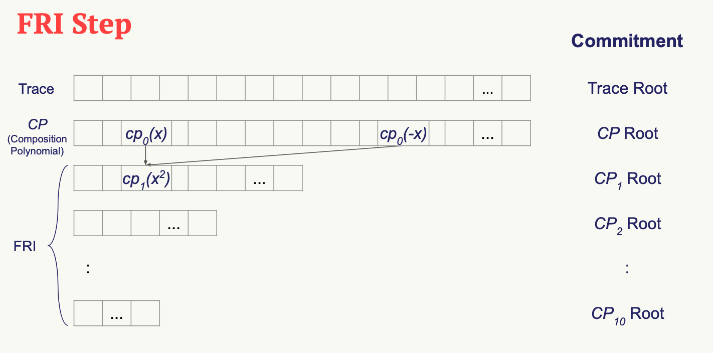
To obtain each layer we need:

To generate a domain for the layer (from the previous layer’s domain).
To generate a polynomial for the layer (from the previous layer’s polynomial and domain).
To evaluate said polynomial on said domain - this is the next FRI layer.

Domain Generation

The first FRI domain is simply the eval_domain that you already generated in Part 1, namely a coset of a group of order 8192. Each subsequent FRI domain is obtained by taking the first half of the previous FRI domain (dropping the second half), and squaring each of its elements.

Formally - we got eval_domain by taking:

$$w, w\cdot h, w\cdot h^2, …, w\cdot h^{8191}$$

The next layer will therefore be:

$$w^2, (w\cdot h)^2, (w\cdot h^2)^2, …, (w\cdot h^{4095})^2$$

Note that taking the squares of the second half of each elements in eval_domain yields exactly
the same result as taking the squares of the first half. This is true for the next layers as well.

Similarly, the domain of the third layer will be:

$$w^4, (w\cdot h)^4, (w\cdot h^2)^4, …, (w\cdot h^{2047})^4$$

And so on.

FRI Folding Operator

The first FRI polynomial is simply the composition polynomial, i.e., cp.

Each subsequent FRI polynomial is obtained by:

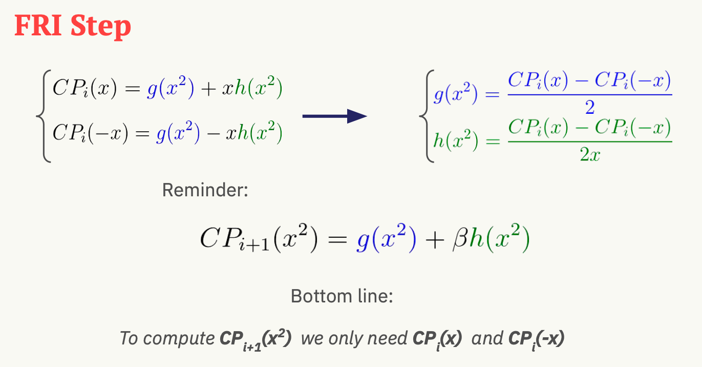
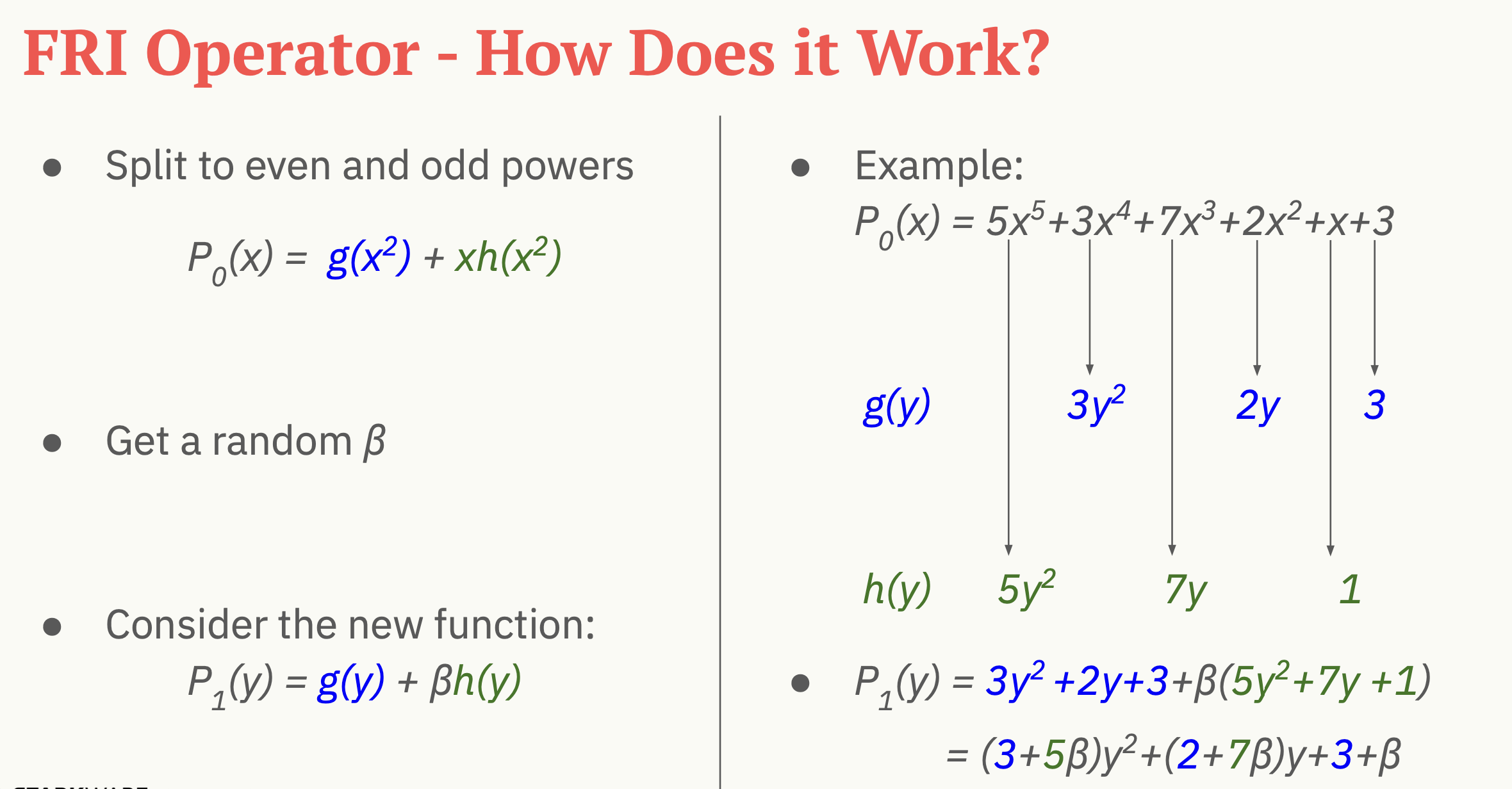
Getting a random field element $\beta$ (by calling Channel.receive_random_field_element).
Multiplying the odd coefficients of the previous polynomial by $\beta$.
Summing together consecutive pairs (even-odd) of coefficients.

Formally, let’s say that the k-th polynomial is of degree $< m$ (for some $m$ which is a power of 2):

$$p_{k}(x) := \sum _{i=0} ^{m-1} c_i x^i$$

Then the (k+1)-th polynomial, whose degree is $< \frac m 2 $ will be:

\[ p_{k+1}(x) := \sum_{i=0} ^{ m / 2 - 1 } (c_{2i} + \beta \cdot c_{2i + 1}) x^i \]

fri

fri example

Generating FRI Commitments

We have now developed the tools to write the FriCommit method, that contains the main FRI commitment loop.

It takes the following 5 arguments:

The composition polynomial, that is also the first FRI polynomial, that is - cp.
The coset of order 8192 that is also the first FRI domain, that is - eval_domain.
The evaluation of the former over the latter, which is also the first FRI layer , that is - cp_eval.
The first Merkle tree (we will have one for each FRI layer) constructed from these evaluations, that is - cp_merkle.
A channel object, that is channel.

The method accordingly returns 4 lists:

The FRI polynomials.
The FRI domains.
The FRI layers.
The FRI Merkle trees.

The method contains a loop, in each iteration of which we extend these four lists, using the last element in each.
The iteration should stop once the last FRI polynomial is of degree 0, that is - when the last FRI polynomial is just a constant. It should then send over the channel this constant (i.e. - the polynomial’s free term).
The Channel class only supports sending strings, so make sure you convert anything you wish to send over the channel to a string before sending.

commitment

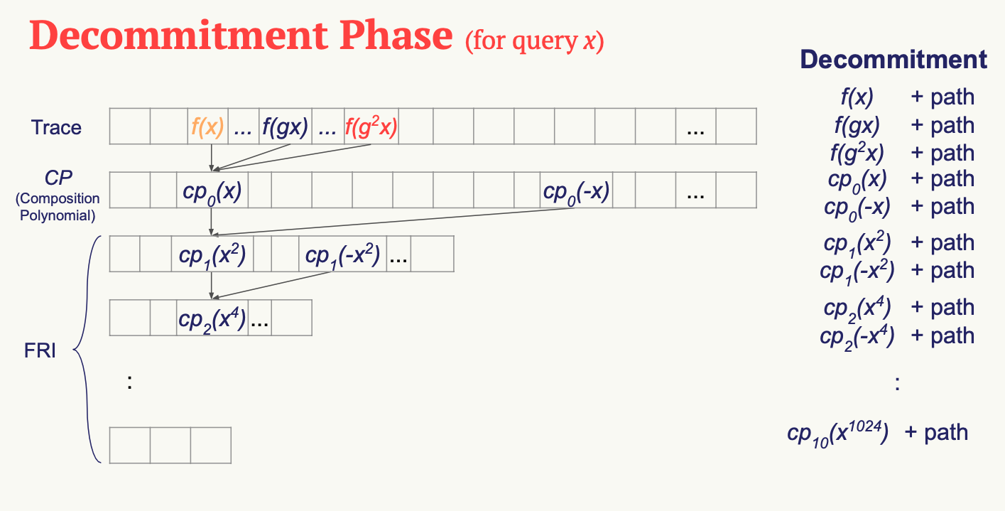
Query Phase

Get q random elements, provide a valdiation data for each

decommitment

references

2023-11-01

understanding plonk

introduction

PLONK, standing for the unwieldy quasi-backronym “Permutations over Lagrange-bases for Oecumenical Noninteractive arguments of Knowledge”. PLONK still requires a “universal and updateable” trusted setup, meaning each program share the same setup. Secondly, there is a way for multiple parties to participate in the trusted setup such that it is secure as long as any one of them is honest.

preliminary

observation 1

a key fact: for non-zero $ f \in \mathbb{F_p}^{\le d}[X]$

for $ r \leftarrow \mathbb{F_p}: Pr[f(r) = 0] \le d/p$
understanding: polynomial $f$ contains at most $d$ roots of zeros.

suppose $ p \approx 2^{256}$ and $ d \approx 2^{40}$ then $d/p$ is negligible.

Therefore, for random $ r \leftarrow \mathbb{F_p}$ if $f(r) = 0$ then $f$ is identically zero w.h.p (with high probability)

=> a simple zero test for a committed polynomial
Note SZDL lemma: this also holds for multivariate polynomials (where d is total degree of f)

observation 2

let $f,g \in \mathbb{F_p}^{\le d}[X]$.
for $ r \leftarrow \mathbb{F_p}$, if $f(r) = g(r)$, then $f = g$ w.h.p

$f(r)-g(r)=0$ => $f-g=0$ w.h.p

=> a simple equality test for two committed polynomials

useful proof gadgets

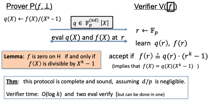
1. zero test

let $ \omega \in \mathbb{F_p} $ be a primitive k-th root of unity $( \omega ^{k} = 1)$
set $ H:= \{1,\omega,\omega^2,\omega^3,…,\omega^{k-1}\} \subseteq \mathbb{F_p} $
let $ f \in \mathbb{F_p}^{\le d}[X]$ and $ b, c \in \mathbb{F_p}$ $(d \ge k)$

task: prove that $f$ is identically zero on $H$
zero test

info the box of $f$ means the commitment of polynomial $f$, i.e $com_f$

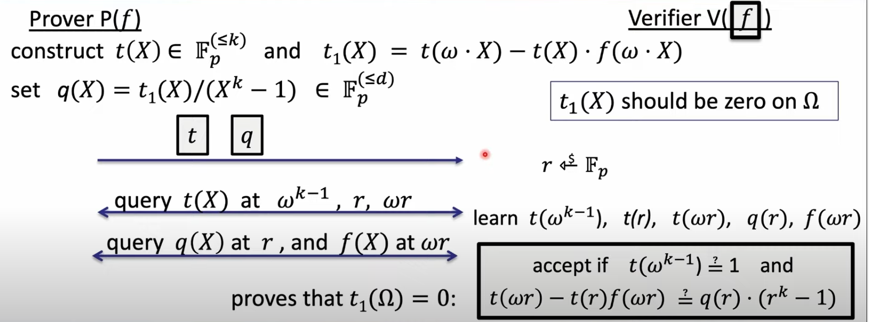
2. product check

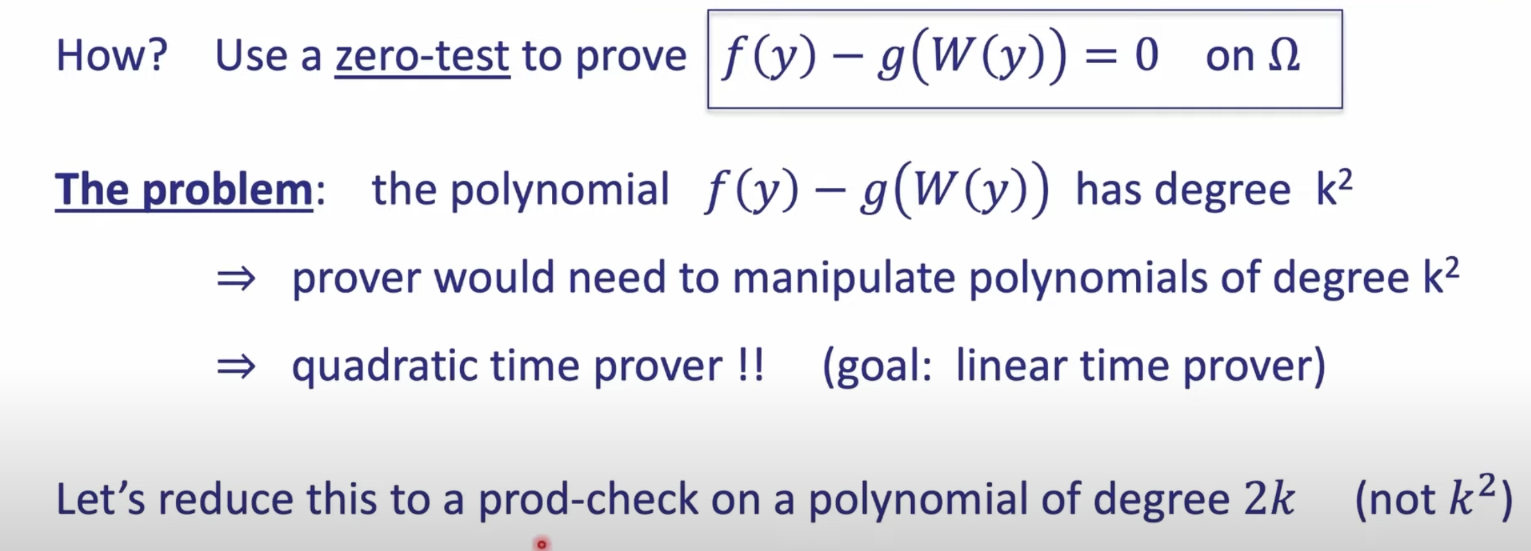
product check on $\Omega: \quad \prod_{a\in \Omega} f(a) = 1$
Set $ t \in \mathbb{F_p}^{\le k}[X]$ to be the degree-k polynomial:
\[ t(1) = f(\omega^0) = f(1), \quad t(\omega^s) = \prod_{i=0}^{s}f(\omega^{i}) \quad for \quad s = 1,…, k-1\]
Then
$t(\omega) = f(1) \cdot f(\omega), \quad t(\omega^2) = f(1) \cdot f(\omega) \cdot f(\omega^2), … $
$t( \omega^{k-1}) = \prod_{a \in \Omega}f(a) = 1$
and $ t(\omega \cdot x) = t(x) \cdot f(\omega \cdot x) $ for all $x \in \Omega $ (including at $x = \omega^{k-1}$)
prod_check_lemma
prod_check_prove_and_verify

Same works for rational functions: $ \prod_{a \in \Omega}{f/g}(a) =1 $
The proof is similar

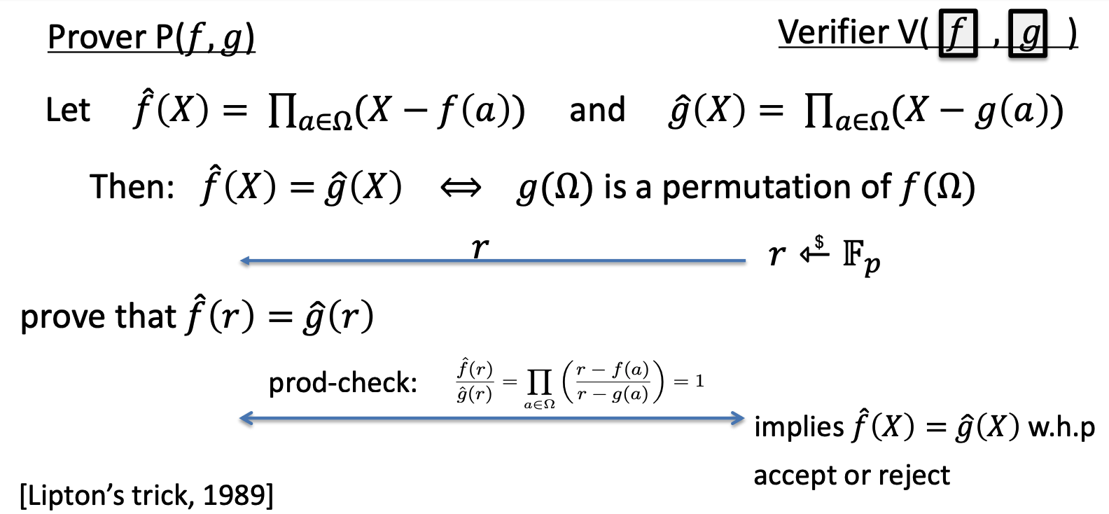
3. permutation check

let $f,g$ be polynomials in $\mathbb{F_p}^{\le d}[X]$. Verifier has $com_f, com_g$.
Prover wants to prove that $(f(1),f(\omega^1),f(\omega^2),…,f(\omega^{k-1})) \in \mathbb{F_p}^{\le k}[X]$ is a permutaion of $(g(1),g(\omega^1),g(\omega^2),…,g(\omega^{k-1})) \in \mathbb{F_p}^{\le k}[X]$

permutation check

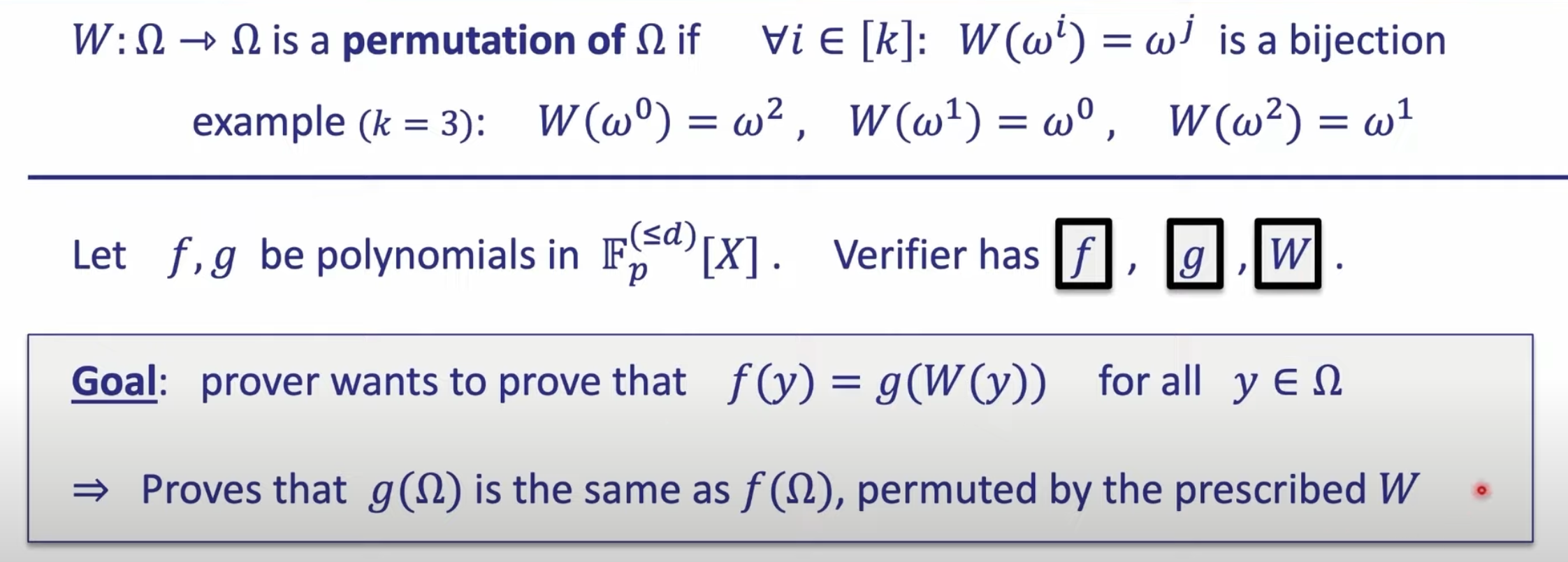
4. prescribed permutation check

PLONK: a poly-IOP for a general circuit C(x,w)

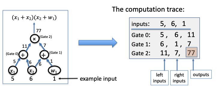
step 1: compile circuit to a computation trace (gate fan-in = 2)

circuit to trace

and encode the trace as polynomial
let $|C|$ be the total number of gates, $|I| := |I_x| + |I_w|$ be total number of inputs, where $|I_x|$ is the number of public inputs, $I_w$ is the number of private inputs.
Let $d=3*|C|+|I|$ and $ \Omega=\{1,\omega,\omega^2,\omega^3,…,\omega^{d-1}\} $

prover interpolates $ T \in \mathbb{F_p}^{\le d}[X]$ such that

T encodes all inputs: $ T(\omega^{-j}) $= input #j, for j = 1,…,|I|
T encodes all wires:
$LeftInput=f(\omega^{3l})$, $ RightInput=f(\omega^{3l+1})$, $Output=f(\omega^{3l+2})$, for $l = 0,1,…, |C| -1$
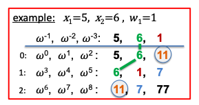
For the example,
inputs
$x_1= 5 = T(\omega^9)$, $x_2= 6 = T(\omega^{10})$, and $w_1 = 1=T(\omega^{11})$
wires
$5=T(\omega^0)$, $6=T(\omega^{1})$, and $11=T(\omega^{2})$
$6=T(\omega^3)$, $1=T(\omega^{4})$, and $7=T(\omega^{5})$
$11=T(\omega^6)$, $7=T(\omega^{7})$, and $77=T(\omega^{8})$

step 2: proving validity of T

Prover needs to prove 4 things

$T(x)$ encodes the correct public inputs
Both prover and verifier interpolate a polynomial $ v(x) \in \mathbb{F_p}^{\le |I_x|}[X]$
that encodes the $x$-inputs to the circuit:
$v(\omega^{-j}) =$ input #j, for $j = 1, …, |I_x|$
In our example, $v(\omega^{-1} = 5), v(\omega^{-2} = 6)$
Let $ \Omega_{inp}=\{\omega^{-1},\omega^{-2},…,\omega^{-|I_x|}\} $
Prover proves by using a ZeroTest on $\Omega_inp$ to prove that
\[T(y) - v(y) =0 \quad \forall y \in \Omega_{inp}\]
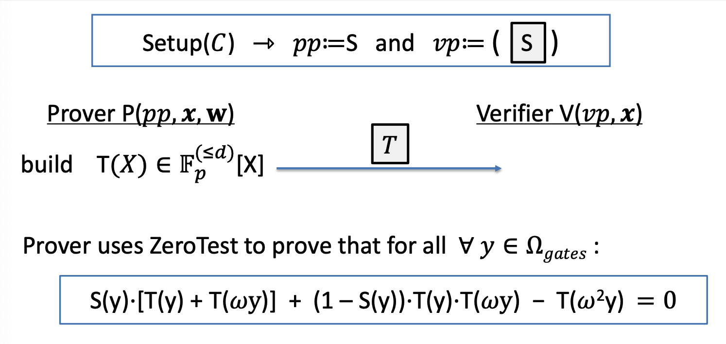
every gate is evaluated correctly
Idea encode gate types using a selector polynomial $S(X)$
define $S(X) \in \mathbb{F_p}^{\le d}[X]$ such that $ \forall l = 0, …, |C| -1$:

$S(\omega^{3l}) =1$ if gate #l is an addition gate
$S(\omega^{3l}) =0$ if gate #l is a multiplication gate

Then, $ \forall y \in \Omega_{gates} : = \{1,\omega^{3},\omega^{6},…,\omega^{3(|C|-1)}\} $
$S(y) \cdot [T(y) + T(\omega y)] + (1-S(y))\cdot T(y) \cdot T(\omega y) = T(\omega^2 y)$
gate_evaluation_zero_test

the wiring is implemented correctly (coppy constraint)

$T(\omega^9,\omega^0)=\sigma(\omega^0,\omega^9)$
$T(\omega^{10},\omega^1,\omega^3)=\sigma(\omega^1,\omega^3,\omega^{10})$
$T(\omega^2,\omega^6)=\sigma(\omega^6,\omega^2)$
$T(\omega^{11},\omega^4)=\sigma(\omega^4,\omega^{11})$
$T(\omega^{5},\omega^7)=\sigma(\omega^7,\omega^{5})$
note: 9 is actually -1, 10 is -2, 11 is -3
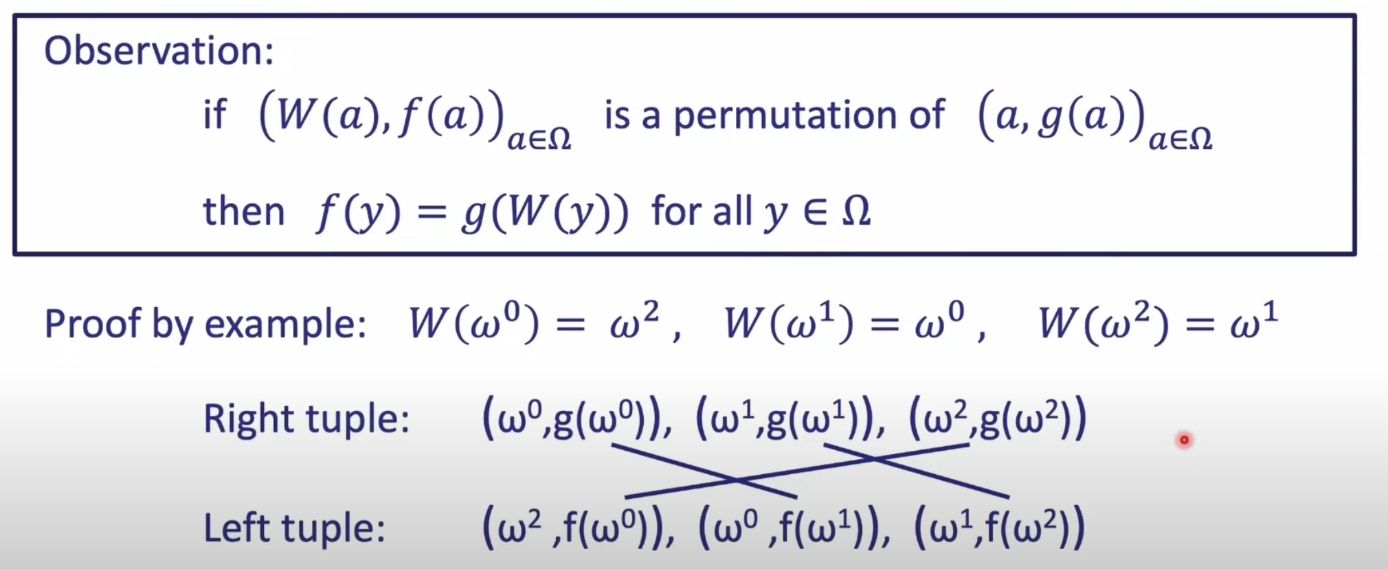
Define a polynomial $W: \Omega -> \Omega$ that implemnets a rotation
$ W(\omega^{10}, \omega^1, \omega^3) =(\omega^1, \omega^3, \omega^{10}) $, $W(\omega^{9}, \omega^0)=(\omega^0, \omega^{9})$, …

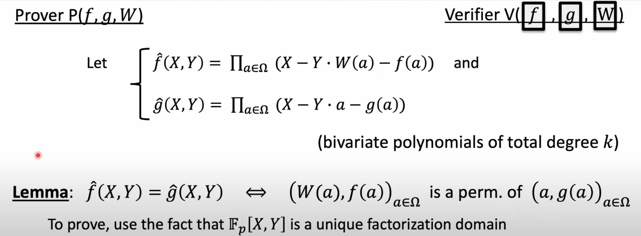
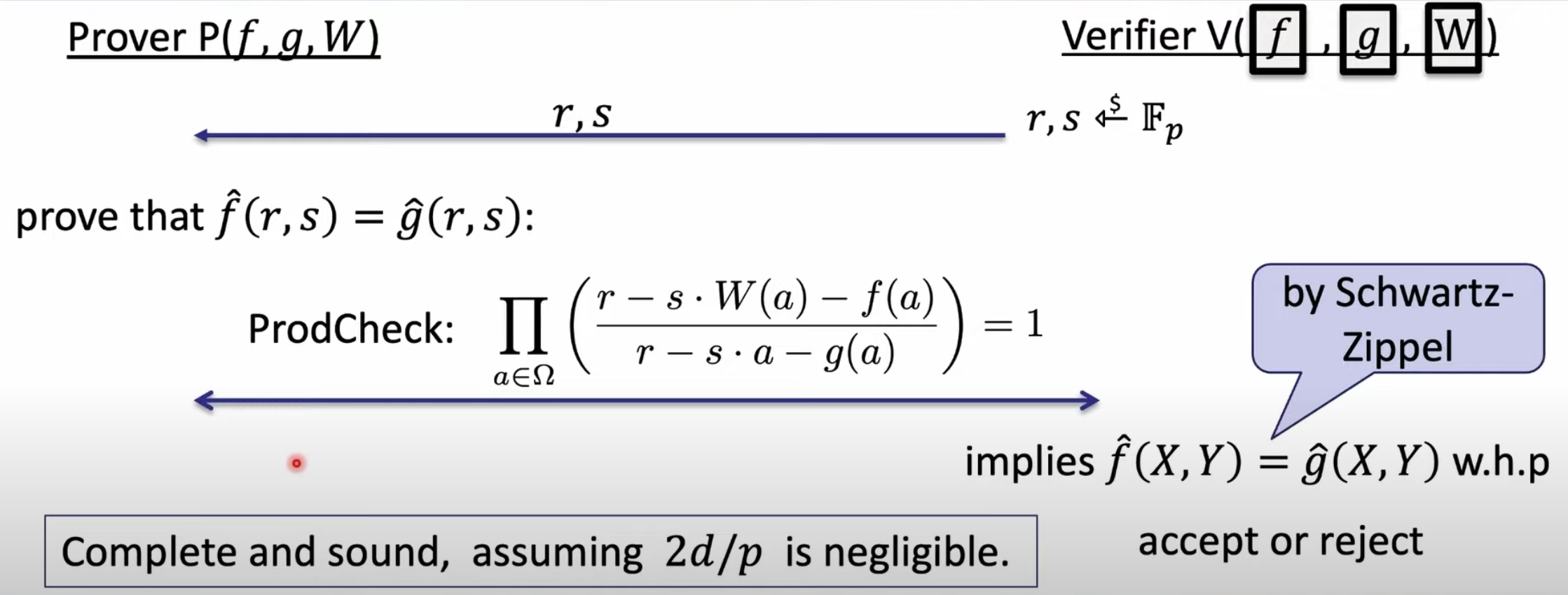
Lemma: $\forall y \in \Omega: T(y) = T(W(y))$ => wire constraints are satisfied
This could be proved using a prescribed permutation check

the output of last gate is 0
this is to prove $T(\omega^8) -77 = 0$

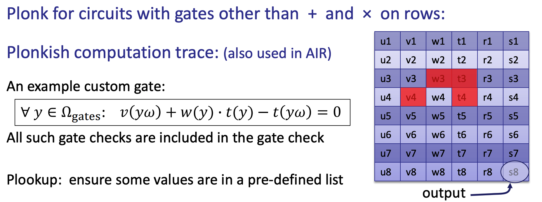
custom gate

$u, v, w, t, r$ are polynomials represent input variables (row number is the gate number). in the Add, Mul only circuits, there are only two inputs, namely LeftInput and RightInput. Hoever, here there are multiple inputs for custom gate.

In the above example, it is a constraint for $ v_4 + w_3 \cdot t_3 - t_4 = 0 $

plonkup

plonkup is to ensure some values are in a pre-defined list. for example

x1	x2	x3	Output
$a_{1,1}$	$a_{1,2}$	$a_{1,3}$	$a_{1,4}$
$a_{2,1}$	$a_{2,2}$	$a_{2,3}$	$a_{2,4}$
…	…	…	…
$a_{n,1}$	$a_{n,2}$	$a_{n,3}$	$a_{n,4}$

$n$ is gate number. the task is to prove a vector

references

2023-10-12

danksharding

introduction

Danksharding is central to Ethereum’s rollup-centric roadmap. The idea is to provide space for large blobs of data, which are verifiable and available, without attempting to interpret them.

Preliminaries

All references to EC, in this report, refer to BLS12_381 [1]. We are mainly concerned with the EC Abelian-group $\mathbb{G_{1}}$ and the EC scalar-field $F_r$. Both are of size $r < 2256$. Note that $2^{32}$ divides the size of the multiplicative-group in $F_r$

Data organization

The input data consists of n = 256 shard-blobs. Each shard-blob is a vector of m = 4096 field-elements referred-to as symbols. The data symbols are organized in an n × m input
matrix
\[
\tag{1}
D_{n x m}^{in} =
\begin{bmatrix}
\displaylines{
d(0,0) & d(0,1) & \dots & d(0,m-1)\\
d(1,0) & d(1,1) & \dots & d(1,m-1)\\
\vdots & \vdots & \ddots & \vdots\\
d(n-1,0) & d(n-1,1) & \dots & d(n-1,m-1)
}
\end{bmatrix}
\]
where each row is one of the shard-blob vectors [2]
In order to enable interpolation and polynomial-commitment to the data, we will pro-
ceed to treat the data symbols as polynomial evaluations.

Let us thus associate each domain location in the input matrix with a field-element pair $u_{\mu}, \omega_{\eta}$, where $\mu \in [0, n−1], \eta \in [0, m−1]$ correspond to the row and column indexes, respectively.The row field-element is defined as $ u_{\mu} \equiv u^{rbo(\mu)}$, where u is a 2n’th root-of-unity such that $u^{2n} = 1$. The column field-element is defined as $ \omega_{\eta} \equiv \omega^{rbo(\eta)}$, where $\omega$ is a 2m’th root-of-unity such that $\omega^{2m} = 1$. Using reverse-bit-order ordering rather than natural-ordering allows accessing cosets in block (consecutive) rather than interleaved manner

coefficients extraction

Taking the data symbols to be evaluations of a 2D-polynomial or 1D-product-polynomials with row degree n−1 and column degree m−1 uniquely defines the polynomials’ coefficients.

2D coeficients extraction

The 2D-polynomial representing the input data can be expressed as
\[\tag{2} d(x,y) \equiv \sum_{i=0}^{n-1}\sum_{j=0}^{m-1} \hat{c}[i,j] x^{i}y^{j}\]
Plugging an evaluation from (1) into (2) results in the following:

\[\tag{3} d(u_{\mu},\omega_{\eta}) \equiv \sum_{i=0}^{n-1}\sum_{j=0}^{m-1} \hat{c}[i,j] {u_{\mu}}^{i}{\omega_{\eta}}^{j}\]

references

[1] Ben Edgington. Bls12-381 for the rest of us. https://hackmd.io/@benjaminion/bls12-381.
[2] Dankrad Feist. Data availability encoding. https://notes.ethereum.org/@dankrad/danksharding_encoding

2023-10-12

fourier series, DFT and FFT

Fourier Series

innter product of two functions

\[ <f(x), g(x)> = \int_{a}^{b} f(x) \bar{g}(x)dx\]
$\bar{g}$ is the congugate of g on complex number system

Fourier series definition

let $f(x)$ be a periodic function over a period of $[-\pi, +\pi]$
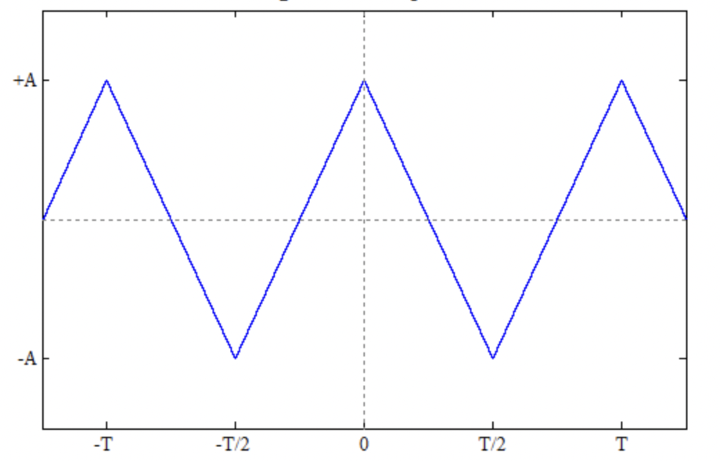
$f(x)$

$ f(x) $ can be transformed into below
\[ f(x) = \frac{A_{0}}{2} + \sum_{k=1}^{\infty}A_{k}cos(kx) + B_{k}sin(kx)\],
where
\[ A_{k} = \frac{1}{\pi} \int_{-\pi}^{+\pi} f(x)cos(kx)dx = \frac{1}{||cos(kx)||^2}<f(x),cos(kx)> \]
\[ B_{k} = \frac{1}{\pi} \int_{-\pi}^{+\pi} f(x)sin(kx)dx = \frac{1}{||sin(kx)||^2}<f(x),sin(kx)> \]
where $A_{k}, B_{k}$ is just the innver product of $f(x)$, and $ cos(kx) $, $sin(kx)$ respectively. intuitively, it is the projection of $f(x)$ over $sin(kx)$, or $cos(kx)$.

if period is L

\[ f(x) = \frac{A_{0}}{2} + \sum_{k=1}^{\infty}A_{k}cos(\frac{2\pi kx}{L}) + B_{k}sin(\frac{2\pi kx}{L})\],
where
\[ A_{k} = \frac{2}{L} \int_{0}^{L} f(x)cos(\frac{2\pi kx}{L})dx\]
\[ B_{k} = \frac{2}{L} \int_{0}^{L} f(x)sin(\frac{2\pi kx}{L})dx\]

Complex Fourier Series

let’s define \[ \psi_k = e^{ikx} = cos(kx) + i \cdot sin(kx)\]
we can prove that $\psi_k, and \psi_j$ are orthogonal as their inner product is zero
proof
\[ <\psi_j, \psi_k> = \int_{-\pi}^{+\pi} e^{jkx}e^{-ikx}dx = \int_{-\pi}^{+\pi} e^{j(j-k)x}dx = \frac{1}{i(j-k)}[e^{i(j-k)x}]_{-\pi}^{\pi}\]
it is 0 if $j \ne k$ , $2\pi $ if $j=k$

note conjugate of $\psi_k$ is $e^{-ikx}$

$f(x) = \frac{1}{2\pi} \sum_{k=-\infty}^{\infty} c_k \psi_k$, where $c_k=<f(x), \psi_k> = \int_{-\pi}^{+\pi} f(x)e^{-ikx}dx$

Discrete Fourier Transform (DFT)

The discrete Fourier transform transforms a sequence of N complex numbers
\[\lbrace x_{n} \rbrace := x_0, x_1,…, x_{N-1} \] into another sequence of complex numbers,
\[\lbrace X_{k} \rbrace := X_0, X_1,…, X_{N-1} \] which is defined by
\[X_{k} = \sum_{n=0}^{N-1} x_{n} \cdot e^{-\frac{i2\pi}{N}kn}\]

let the n-th root of unity be $\omega_N = e^{-\frac{2\pi i}{N}}$, we have
\[ \tag{1.1} X_{k} = \sum_{n=0}^{N-1} x_{n} \cdot \omega_N^{kn}\]

inverse DFT

The inverse transform is given by
\[ \tag{1.2} x_{n} = \frac{1}{N}\sum_{k=0}^{N-1} X_{k} \cdot \omega_N^{-kn}\]

the unitary DFT

Another way of looking at the DFT is to note that the DFT can be expressed as the DFT matrix, a Vandermonde matrix, introduced by Sylvester in 1867.
\[
\boldsymbol{F} =
\begin{bmatrix}
\displaylines{
\omega_{N}^{0\cdot0} & \omega_{N}^{0\cdot1} & \dots & \omega_{N}^{0\cdot (N-1)}\\
\omega_{N}^{1\cdot0} & \omega_{N}^{1\cdot1} & \dots & \omega_{N}^{2\cdot (N-1)}\\
\vdots & \vdots & \ddots & \vdots\\
\omega_{N}^{N-1\cdot0} & \omega_{N}^{N-1\cdot1} & \dots & \omega_{N}^{N-1\cdot (N-1)}
}
\end{bmatrix}
\]
where $ \omega_{N} = e^{-\frac{i2\pi}{N}}$ is a primitive Nth root of unity. (any complex number that yields 1 when raised to some positive integer power n)

\[ X = F \cdot x^{T}\]
$x$ is a column vector

Polynomial & DFT

Polynomial evaluation & DFT

let a polynomial be
$$f(x)=\sum_{n=0}^{N-1}x_nx^n$$
then,
$$f(\omega_N^{k})=\sum_{n=0}^{N-1}x_n\omega_N^{kn},\quad k=0,1,2,…,N-1$$
compare this equation with E.q(1.1), we can know that DFT is the evaluations of a polynomial at N points of Nth root of unity, $\omega_N^{0},\omega_N^1,\omega_N^2,…,\omega_N^{N-1}$

$$(\omega_N^{0},X_0),(\omega_N^1,X_1),(\omega_N^2,X_2),…,(\omega_N^{N-1},X_{N-1})$$

Polynomial interpolation & IDFT

According to E.q(1.2), IDFT is the polynomial interpolation (getting original polynomial coefficients).

Fast Fourier Transform (FFT) [3]

The problem is to calculate the below
\[ \tag{2.1} X_{k} = \sum_{n=0}^{N-1} x_{n} \cdot \omega_N^{kn}, \quad k= 0,1,…,N-1\]
A straightforward calculation using would require $N^2$ operations where “operation” means, as it will throughout this note, a complex multiplication followed by a complex addition.
The FFT algorithm described here iterates on the array and yields the result in less than $ 2N log_2N $

To derive the algorithm, suppose $N$ is a composite, i.e., $N = r_1\cdot r_2$. Then let the indices in (2.1) be expressed
\[ k = k_1r_1 + k_0, \quad k_0 = 0,1,…,r_1-1, \quad k_1 = 0,1,…, r_2 -1 \]
\[ n = n_1r_2 + n_0, \quad n_0 = 0,1,…,r_2-1, \quad n_1 = 0,1,…, r_1 -1 \]

Since $ n = n_1r_2 + n_0$, we can write

\[ \tag{2.2} X(k_1, k_0) = \sum_{n_0} \sum_{n_1}x(n_1,n_0)\omega_N^{kn} = \sum_{n_0} \sum_{n_1}x(n_1,n_0)\omega_N^{kn_1r_2}\omega_N^{kn_0} \]
note $ x(n_1,n_0)$ is same to $x(n)$, just the indexing is transformed form 1D to 2D. You can think original 1D array of size N is resized to a matrix of size $ (r_2, r_1) $, $r_1$ is number of cols, while $r_2$ is number of rows

Since $k = k_1r_1 + k_0$, we have
\[ \omega_N^{kn_1r_2} =\omega_N^{(k_1r_1+k_0)n_1r_2} = \omega_N^{(k_1r_1)n_1r_2} \cdot \omega_N^{k_0n_1r_2}\]
according to the property of Nth root of unity, $ \omega_N^{N} = \omega_N^{r_1r_2} =1 $, $ \omega_N^{(k_1r_1)n_1r_2}$ is also 1.
then we have
\[ \omega_N^{kn_1r_2} = \omega_N^{k_0n_1r_2}\]
substitute it into E.q 2.2, we get
\[ \tag{2.3} X(k_1, k_0) = \sum_{n_0} \sum_{n_1}x(n_1,n_0)\omega_N^{kn} = \sum_{n_0} \sum_{n_1}x(n_1,n_0)\omega_N^{k_0n_1r_2}\omega_N^{kn_0} \]
Therefore, the inner sum, over $n_1$, depends only on $k_0$ and $n_0$, and can be defined as a new array,
\[ \tag{2.4} x_1(k_0, n_0) = \sum_{n_1} x(n_1, n_0) \cdot \omega_N^{k_0n_1r_2}\]
E.q(2.3) can be writtern as
\[ \tag{2.5} X(k_1, k_0) = \sum_{n_0} x_1(k_0,n_0)\omega_N^{kn_0} = \sum_{n_0} x_1(k_0,n_0)\omega_N^{(k_1r_1 + k_0)n_0} \]

There are N elements in the matrix $x_1$, each requiring $r_1$ operations, giving a total of $Nr_1$ operations. Similarly, it takes $Nr_2$ operations to calculate $X$ from $x_1$. Therefore, the two-step algorithm, given by Eq(2.4) and Eq(2.5) requires a total of
\[ \tag{2.6} T = N(r_1+r_2) \]

it is easy to see how successive applications of the above procedure (recursively), starting with its appliation to Eq(2.4) give an m-step algorihtm requiring
\[ \tag{2.7} T = N(r_1+r_2 + … + r_m) \]
where
\[ N = \prod_{j=1}^{j=m}r_j\]
if all $r_j$ are equal to $r$, i.e $N = r^m $, which gives $ m = log_rN $
E.q(2.7) becomes
\[ \tag{2.8} T = N(m \cdot r) = rNm = rN(log_rN) \]

radix-2 FFT

The algorithm with $r=2$ is derived by expressing the indices in the form

\[\tag{3.1} k=k_{m-1} \cdot 2^{m-1} + … + k_1 \cdot 2 + k_0 \]
\[\tag{3.2} n=n_{m-1} \cdot 2^{m-1} + … + n_1 \cdot 2 + n_0 \]
where $ k_v \in [0,1] $, for $ v = 0,…,m-1 $, and $ n_v \in [0,1] $, for $ v = 0,…,m-1 $
$k_v$ and $n_v$ are the contents of the respective bit positions in the binary representation of $k$ and $n$

All arrays will now be written as functions of the bits of their indices. With this convention E.q(2.1) is written as
\[ \tag{3.3}
\displaylines{
X(k_{m-1}, …, k_0) = \sum_{n_0}\sum_{n_1} … \sum_{n_{m-1}} x(n_{m-1}, …,n_1, n_0) \cdot \omega_N^{kn} \\
= \sum_{n_0}\sum_{n_1} … \sum_{n_{m-1}} x(n_{m-1}, …,n_1, n_0) \cdot \omega_N^{k(n_{m-1} \cdot 2^{m-1} + … + n_1 \cdot 2 + n_0)} \\
= \sum_{n_0}\sum_{n_1} … \sum_{n_{m-1}} x(n_{m-1}, …,n_1, n_0) \cdot \omega_N^{kn_{m-1} \cdot 2^{m-1} + … + kn_1 \cdot 2 + kn_0}
}
\]
where the sums are over $n_v \in [0,1]$, for $v = 0,1,…,m-1$

Since \[ \displaylines{
\omega_N^{kn_{m-1}\cdot 2^{m-1}} = \omega_N^{(k_{m-1} \cdot 2^{m-1} + … + k_1 \cdot 2 + k_0)n_{m-1}\cdot 2^{m-1}} \\
= \omega_N^{k_0 n_{m-1} \cdot 2^{m-1}}
}
\]
(it is easy to show that all other terms are 1 as $ \omega_N^{2^m} = 1 $, so only $ k_0$ is kept)

the innermost sum of E.q(3.3) over $n_{m-1} $, depends only on $ k_0, n_{m-2}, …, n_0$ and can be writtern
\[ \displaylines{
x_1(k_0, n_{m-2}, …, n_1, n_0) = \sum_{n_{m-1}} x(n_{m-1}, …, n_0) \cdot \omega_N^{k_0 n_{m-1} \cdot 2^{m-1}}
}
\]

proceeding to the next innermost sum, over $ n_{m-2} $, and so on, and using
\[ \displaylines{
\omega_N^{kn_{m-l}\cdot 2^{m-l}} = \omega_N^{(k_{m-1} \cdot 2^{m-1} + … + k_1 \cdot 2 + k_0)n_{m-l}\cdot 2^{m-l}} \\
= \omega_N^{(k_{l-1}\cdot 2^{l-1} + … + k_0) n_{m-l} \cdot 2^{m-1}}
}
\]
one obtains successive arrays
\[\displaylines{
x_l(k_0, …, k_{l-1}, n_{m-l-1}, … , n_0) \\
= \sum_{n_{m-l}}x_{l-1}(k_0, …, k_{l-2}, n_{m-l}, …, n_0 ) \cdot \omega_N^{(k_{l-1}\cdot 2^{l-1} + …+ k_0) \cdot n_{m-l} \cdot 2^{m-l}}
}\]
for $l = 1,2,…,m $

writing out the sum this appears as
\[ \tag{3.4} \displaylines{
x_l(k_0, …, k_{l-1}, n_{m-l-1}, … , n_0) \\
= x_{l-1}(k_0, …, k_{l-2}, 0, n_{m-l -1}, …, n_0 ) \cdot \omega_N^{(k_{l-1}\cdot 2^{l-1} + …+ k_0) \cdot 0 \cdot 2^{m-l}} \\
+ x_{l-1}(k_0, …, k_{l-2}, 1, n_{m-l -1}, …, n_0 ) \cdot \omega_N^{(k_{l-1}\cdot 2^{l-1} + …+ k_0) \cdot 1 \cdot 2^{m-l}} \\
= x_{l-1}(k_0, …, k_{l-2}, 0, n_{m-l -1}, …, n_0 ) \\
+ x_{l-1}(k_0, …, k_{l-2}, 1, n_{m-l-1}, …, n_0 ) \cdot \omega_N^{(k_{l-1}\cdot 2^{l-1} + k_{l-2}\cdot 2^{l-2 }+k_{l-3}\cdot 2^{l-3} + …+ k_0) \cdot 2^{m-l}} \\
= x_{l-1}(k_0, …, k_{l-2}, 0, n_{m-l -1}, …, n_0 ) \\
+ \omega_N^{k_{l-1}\cdot 2^{l-1} \cdot 2^{m-l} } \cdot \omega_N^{k_{l-2}\cdot 2^{l-2 } \cdot 2^{m-l}} \cdot x_{l-1}(k_0, …, k_{l-2}, 1, n_{m-l-1}, …, n_0 ) \cdot \omega_N^{(k_{l-3}\cdot 2^{l-3} + …+ k_0) \cdot 2^{m-l}} \\
= x_{l-1}(k_0, …, k_{l-2}, 0, n_{m-l -1}, …, n_0 ) \\
+ \omega_N^{k_{l-1}\cdot 2^{m-1} } \cdot \omega_N^{k_{l-2}\cdot 2^{m-2}} \cdot x_{l-1}(k_0, …, k_{l-2}, 1, n_{m-l-1}, …, n_0 ) \cdot \omega_N^{(k_{l-3}\cdot 2^{l-3} + …+ k_0) \cdot 2^{m-l}} \\
= x_{l-1}(k_0, …, k_{l-2}, 0, n_{m-l -1}, …, n_0 ) \\
+ (-1)^{k_{l-1} } \cdot i^{k_{l-2}} \cdot x_{l-1}(k_0, …, k_{l-2}, 1, n_{m-l-1}, …, n_0 ) \cdot \omega_N^{(k_{l-3}\cdot 2^{l-3} + …+ k_0) \cdot 2^{m-l}}
}\]
according to the indexing convension, this is stored in a location whose index is
\[ k_0 \cdot 2^{m-1} + … + k_{l-1} \cdot 2 ^{m-l} + n_{m-l-1} \cdot 2^{m-l-1} + … + n_0 \]

It can be seen in E.q(3.4) that only the two storage locations with indices having 0 and 1 in the $2^{m-l}$ bit position are involved in the computation. Parallel computation is permitted since the operation described by E.q(3.4) can be carried out with all values of $k_0, …, k_{l-2} $, and $ n_0, …, n_{m-l-1}$ simultaneously. In some applications it is convenient to use E.q(3.4) to express $x_l$ in terms of $x_{l-2}$, giving what is equivalent to an algorithm with $r = 4$.
the last array calculated gives the desired Fourier sums,

\[\tag{3.5}
X(k_{m-1}, …, k_0) = x_{m}(k_0, …, k_{m-1})
\]
in such an order that the index of an X must have its binary bits put in reverse order to yield its index in the array $x_m$

references

2023-10-01

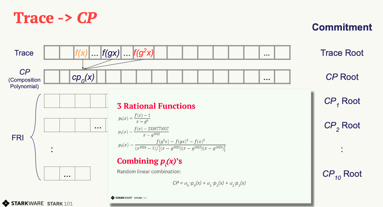
markdown & latex

markdown by example

italic
color

latex by example

symbol

$ \mu $
$ \omega $
$ \sigma $
$ \epsilon $
$ \zeta $
$ \eta $
$ \theta $
$ \kappa $
$ \nu $
$ \omicron $
$ \rho $
$ \delta $
$ \tau $
$ \upsilon $
$ \phi $
$ \chi $
$ \psi $
$\mathcal O$

font & effects

$ \mathbb{G_{1}}$
$ \boldsymbol{F}$
$ \hat{h} $

equation

\[ \tag{1.1} X = F \cdot x^{T}\]

blob

\[
\begin{bmatrix}
\displaylines{
\omega_{N}^{0\cdot0} & \omega_{N}^{0\cdot1} & \dots & \omega_{N}^{0\cdot (N-1)}\\
\omega_{N}^{1\cdot0} & \omega_{N}^{1\cdot1} & \dots & \omega_{N}^{2\cdot (N-1)}\\
\vdots & \vdots & \ddots & \vdots\\
\omega_{N}^{N-1\cdot0} & \omega_{N}^{N-1\cdot1} & \dots & \omega_{N}^{N-1\cdot (N-1)}
}
\end{bmatrix}
\]

2023-07-14

zkp demystify zokrates

pipeline

source file

an example, square.zok

def main(private field a, field b) {
    assert(a * a == b);
    return;
}

The keyword private signals that we do not want to reveal this input, but still prove that we know its value.

compile

1	zokrates compile -i root.zok

after compile, it generates below files

out
out.r1cs
abi.json

setup

Performs a trusted setup for a given constraint system

1	zokrates setup

options

-i, –input Path of the binary [default: out]
it generates below two files
proving.key
verification.key

x1	x2	x3	Output
\(a_{1,1}\)	\(a_{1,2}\)	\(a_{1,3}\)	\(a_{1,4}\)
\(a_{2,1}\)	\(a_{2,2}\)	\(a_{2,3}\)	\(a_{2,4}\)
…	…	…	…
\(a_{n,1}\)	\(a_{n,2}\)	\(a_{n,3}\)	\(a_{n,4}\)