2023-11-03

stark 101

trace and low degree extension

the objective is to develop a STARK prover for the FibonacciSq sequence over a finite field. The FibonacciSq sequence is defined by the recurrence relation
\[ a_{n+2} = a_{n+1} ^2 + a_n ^2 \]

the statement is: I know a FieldElement $X\in \mathbb{F}$ such that the 1023rd element of the FibonacciSq sequence starting with $1, X$ is $2338775057$

The underlying field of this class is $\mathbb{F}_{3221225473}$ ($3221225473 = 3 \cdot 2^{30} + 1$), so all operations are done modulo 3221225473.

FibonacciSq Trace

let’s construct a list a of length 1023, whose first two elements will be FieldElement objects representing 1 and 3141592, respectively. The next 1021 elements will be the FibonacciSq sequence induced by these two elements. a is called the trace of FibonacciSq, or, when the context is clear, the trace.

Thinking of Polynomials

We now want to think of the sequence as the evaluation of some polynomial $f$ of degree 1022.
We will choose the domain to be some subgroup $G \subseteq \mathbb{F}^\times$ of size 1024, for reasons that will become clear later.

(Recall that $\mathbb{F}^\times$ denotes the multiplicative group of $\mathbb{F}$, which we get from $\mathbb{F}$ by omitting the zero element with the induced multiplication from the field. A subgroup of size 1024 exists because $\mathbb{F}^\times$ is a cyclic group of size $3\cdot 2^{30}$, so it contains a subgroup of size $2^i$ for any $0 \leq i \leq 30$).

Find a Group of Size 1024

If we find an element $g \in \mathbb{F}$ whose (multiplicative) order is 1024, then $g$ will generate such a group. Create a list called G with all the elements of $G$, such that $G[i] := g^i$.

Evaluating on a Larger Domain

then, interpolating G over a we get a polynomial f. The trace, viewed as evaluations of a polynomial $f$ on $G$, can now be extended by evaluating $f$ over a larger domain, thereby creating a Reed-Solomon error correction code.

Cosets

To that end, we must decide on a larger domain on which $f$ will be evaluated. We will work with a domain that is 8 times larger than $G$.
A natural choice for such a domain is to take some group $H$ of size 8192 (which exists because 8192 divides $|\mathbb{F}^\times|$), and shift it by the generator of $\mathbb{F}^\times$, thereby obtaining a coset of $H$.

Create a list called H of the elements of $H$, and multiply each of them by the generator of $\mathbb{F}^\times$ to obtain a list called eval_domain. In other words, eval_domain = $\{w\cdot h^i | 0 \leq i <8192 \}$ for $h$ the generator of $H$ and $w$ the generator of $\mathbb{F}^\times$.

Evaluate on a Coset

1 2	f = interpolate_poly(G[:-1], a) f_eval = [f(d) for d in eval_domain]

Commitments

We will use Sha256-based Merkle Trees as our commitment scheme.

1 2	from merkle import MerkleTree f_merkle = MerkleTree(f_eval)

Channel

Theoretically, a STARK proof system is a protocol for interaction between two parties - a prover and a verifier. In practice, we convert this interactive protocol into a non-interactive proof using the Fiat-Shamir Heuristic. In this tutorial you will use the Channel class, which implements this transformation. This channel replaces the verifier in the sense that the prover (which you are writing) will send data, and receive random numbers or random FieldElement instances.

constraints

In this part, we are going to create a set of constraints over the trace a.

Step 1 - FibonacciSq Constraints

For a to be a correct trace of a FibonacciSq sequence that proves our claim:

The first element has to be 1, namely $a[0] = 1$.
The last element has to be 2338775057, namely $a[1022] = 2338775057$.
The FibonacciSq rule must apply, that is - for every $i<1021$, $a[i+2]=a[i+1]^2+a[i]^2$.

Step 2 - Polynomial Constraints

Recall that f is a polynomial over the trace domain, that evaluates exactly to a over $G \setminus {g^{1023}}$ where $G={g^i : 0\leq i\leq 1023}$ is the “small” group generated by $g$.

We now rewrite the above three constraints in a form of polynomial constraints over f:

$a[0] = 1$ is translated to the polynomial $f(x) - 1$, which evalutes to 0 for $x = g^0$ (note that $g^0$ is $1$).
$a[1022] = 2338775057$ is translated to the polynomial $f(x) - 2338775057$, which evalutes to 0 for $x = g^{1022}$.
$a[i+2]=a[i+1]^2+a[i]^2$ for every $i<1021$ is translated to the polynomial $f(g^2 \cdot x) - (f(g \cdot x))^2 - (f(x))^2$, which evaluates to 0 for $x \in G \backslash {g^{1021}, g^{1022}, g^{1023}}$.

Step 3 - Rational Functions (That are in Fact Polynomials)

Each of the constraints above is represented by a polynomial $u(x)$ that supposedly evaluates to $0$ on certain elements of the group $G$. That is, for some $x_0, \ldots, x_k \in G$, we claim that

\[u(x_0) = \ldots = u(x_k) = 0\]

(note that for the first two constaints, $k=0$ because they only refer to one point and for the third $k=1021$).

This is equivalent to saying that $u(x)$ is divisible, as a polynomial, by all of ${(x-x_i)}_{i=0}^k$, or, equivalently, by

\[\prod_{i=0}^k (x-x_i)\]

Therefore, each of the three constraints above can be written as a rational function of the form:

\[\frac{u(x)}{\prod_{i=0}^k (x-x_i)}\]

for the corresponding $u(x)$ and ${x_i}_{i=0}^k$. In this step we will construct these three rational functions and show that they are indeed polynomials.

The First Constraint:

In the first constraint, $f(x) - 1$ and ${x_i} = {1}$.

We will now construct the polynomial $p_0(x)=\frac{f(x) - 1}{x - 1}$, making sure that $f(x) - 1$ is indeed divisible by $(x-1)$.

The Second Constraint

Construct the polynomial p1 representing the second constraint, $p_1(x)= \frac{f(x) - 2338775057}{x - g^{1022}}$, similarly:

The Third Constraint - Succinctness

The last constraint’s rational function is slightly more complicated:

\[p_2(x) = \frac{f(g^2 \cdot x) - (f(g \cdot x))^2 - (f(x))^2}{\prod\limits_{i=0}^{1020} (x-g^i)}\]

whose denominator can be rewritten, so that the entire expression is easier to compute:

$$\frac{f(g^2 \cdot x) - (f(g \cdot x))^2 - (f(x))^2}{\frac{x^{1024} - 1}{(x-g^{1021})(x-g^{1022})(x-g^{1023})}}$$

This follows from the equality

$$\prod\limits_{i=0}^{1023} (x-g^i) = x^{1024} - 1$$

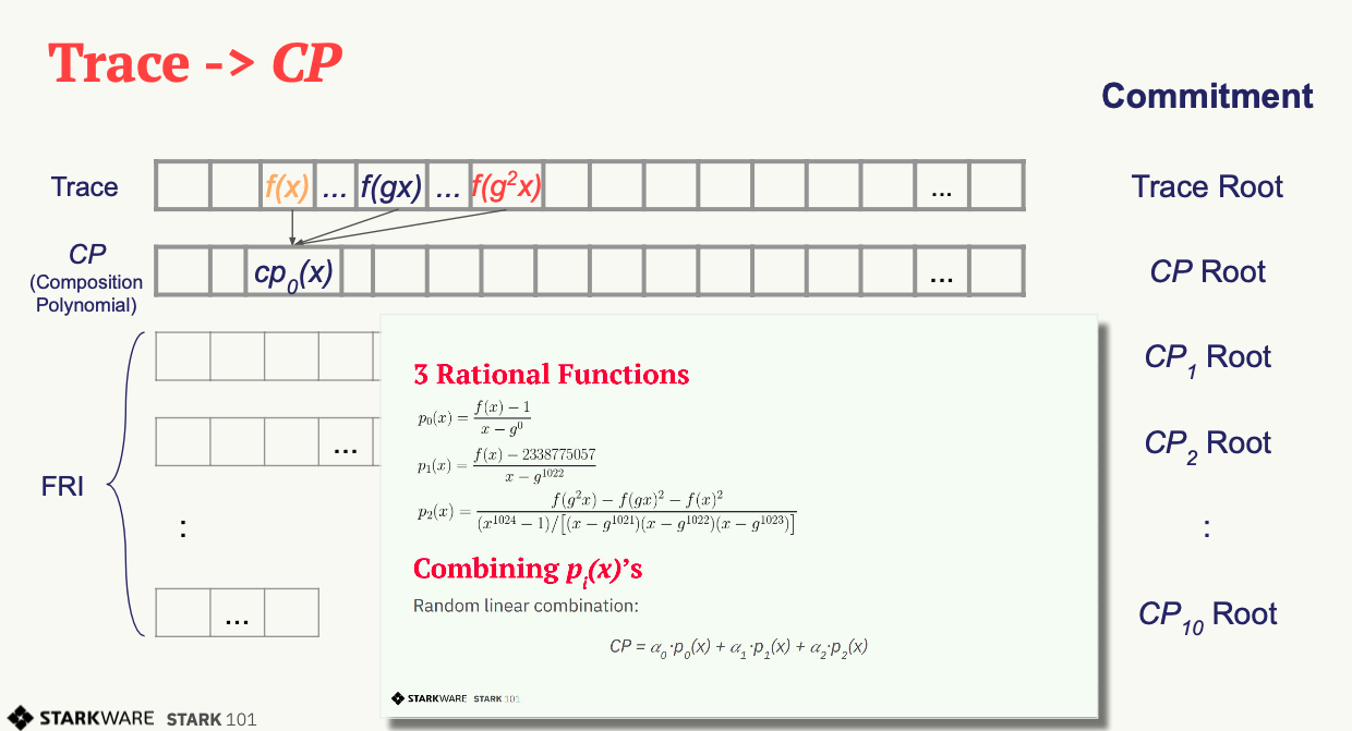
Step 4 - Composition Polynomial

Recall that we’re translating a problem of checking the validity of three polynomial constraints to checking that each of the rational functions $p_0, p_1, p_2$ are polynomials.

Our protocol uses an algorithm called FRI to do so, which will be discussed in the next part.

In order for the proof to be succinct (short), we prefer to work with just one rational function instead of three. For that, we take a random linear combination of $p_0, p_1, p_2$ called the compostion polynomial (CP for short):

$$CP(x) = \alpha_0 \cdot p_0(x) + \alpha_1 \cdot p_1(x) + \alpha_2 \cdot p_2(x)$$

where $\alpha_0, \alpha_1, \alpha_2 $ are random field elements obtained from the verifier, or in our case - from the channel.

Proving that (the rational function) $CP$ is a polynomial guarantess, with high probability, that each of $p_0, p_1, p_2$ are themselves polynomials.

Commit on the Composition Polynomial

Lastly, we evaluate $cp$ over the evaluation domain (eval_domain), build a Merkle tree on top of that and send its root over the channel. This is similar to commiting on the LDE trace, as we did at the end of part 1.

trace to cp

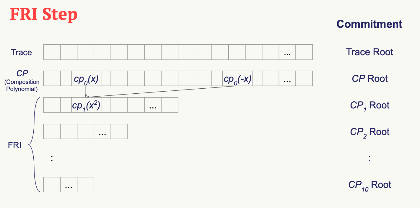
FRI Commitments

FRI Folding

Our goal in this part is to construct the FRI layers and commit on them.

To obtain each layer we need:

To generate a domain for the layer (from the previous layer’s domain).
To generate a polynomial for the layer (from the previous layer’s polynomial and domain).
To evaluate said polynomial on said domain - this is the next FRI layer.

Domain Generation

The first FRI domain is simply the eval_domain that you already generated in Part 1, namely a coset of a group of order 8192. Each subsequent FRI domain is obtained by taking the first half of the previous FRI domain (dropping the second half), and squaring each of its elements.

Formally - we got eval_domain by taking:

$$w, w\cdot h, w\cdot h^2, …, w\cdot h^{8191}$$

The next layer will therefore be:

$$w^2, (w\cdot h)^2, (w\cdot h^2)^2, …, (w\cdot h^{4095})^2$$

Note that taking the squares of the second half of each elements in eval_domain yields exactly
the same result as taking the squares of the first half. This is true for the next layers as well.

Similarly, the domain of the third layer will be:

$$w^4, (w\cdot h)^4, (w\cdot h^2)^4, …, (w\cdot h^{2047})^4$$

And so on.

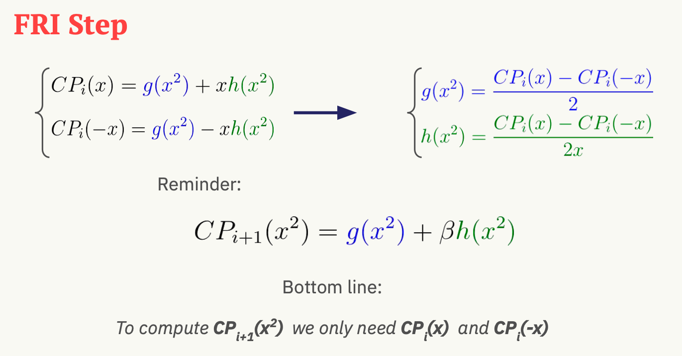
FRI Folding Operator

The first FRI polynomial is simply the composition polynomial, i.e., cp.

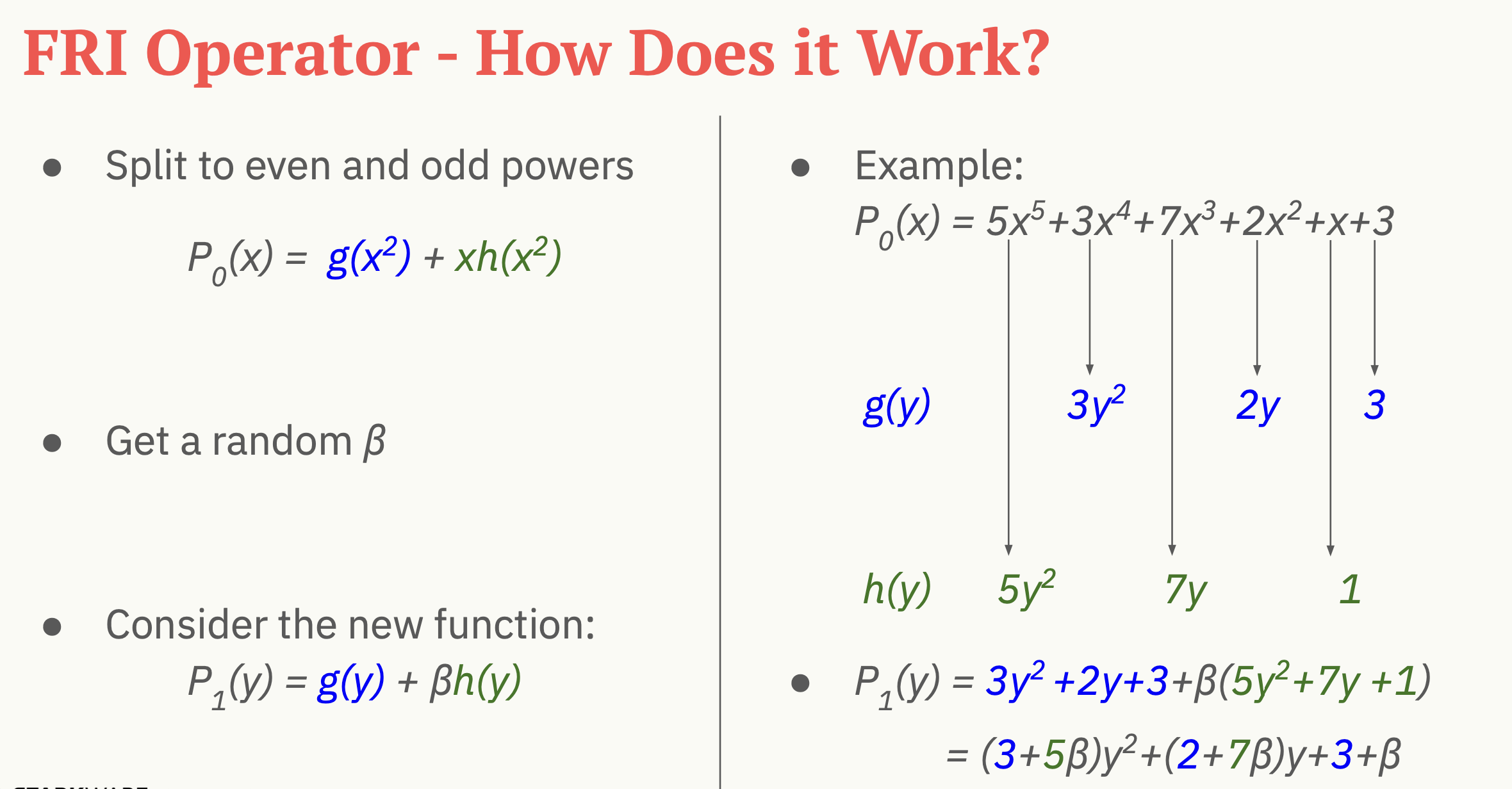
Each subsequent FRI polynomial is obtained by:

Getting a random field element $\beta$ (by calling Channel.receive_random_field_element).
Multiplying the odd coefficients of the previous polynomial by $\beta$.
Summing together consecutive pairs (even-odd) of coefficients.

Formally, let’s say that the k-th polynomial is of degree $< m$ (for some $m$ which is a power of 2):

$$p_{k}(x) := \sum _{i=0} ^{m-1} c_i x^i$$

Then the (k+1)-th polynomial, whose degree is $< \frac m 2 $ will be:

\[ p_{k+1}(x) := \sum_{i=0} ^{ m / 2 - 1 } (c_{2i} + \beta \cdot c_{2i + 1}) x^i \]

fri

fri example

Generating FRI Commitments

We have now developed the tools to write the FriCommit method, that contains the main FRI commitment loop.

It takes the following 5 arguments:

The composition polynomial, that is also the first FRI polynomial, that is - cp.
The coset of order 8192 that is also the first FRI domain, that is - eval_domain.
The evaluation of the former over the latter, which is also the first FRI layer , that is - cp_eval.
The first Merkle tree (we will have one for each FRI layer) constructed from these evaluations, that is - cp_merkle.
A channel object, that is channel.

The method accordingly returns 4 lists:

The FRI polynomials.
The FRI domains.
The FRI layers.
The FRI Merkle trees.

The method contains a loop, in each iteration of which we extend these four lists, using the last element in each.
The iteration should stop once the last FRI polynomial is of degree 0, that is - when the last FRI polynomial is just a constant. It should then send over the channel this constant (i.e. - the polynomial’s free term).
The Channel class only supports sending strings, so make sure you convert anything you wish to send over the channel to a string before sending.

commitment

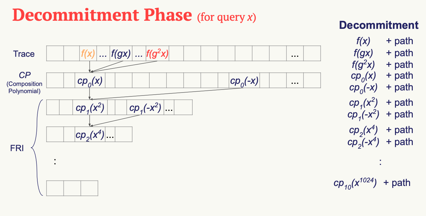
Query Phase

Get q random elements, provide a valdiation data for each

decommitment

cliff's personal blog