introduction
zk-SNARKs cannot be applied to any computational problem directly; rather, you have to convert the problem into the right “form” for the problem to operate on. The form is called a “quadratic arithmetic program” (QAP), and transforming the code of a function into one of these is itself highly nontrivial.
The example that we will choose is a simple one: proving that you know the solution to a cubic equation: \(x^3 + x + 5 == 35\)
Note that modulo (%) and comparison operators (<, >, ≤, ≥) are NOT supported, as there is no efficient way to do modulo or comparison directly in finite cyclic group arithmetic (be thankful for this; if there was a way to do either one, then elliptic curve cryptography would be broken faster)
You can extend the language to modulo and comparisons by providing bit decompositions (eg. \(13 = 2^3 + 2^2 + 1\)) as auxiliary inputs, proving correctness of those decompositions and doing the math in binary circuits; in finite field arithmetic, doing equality (==) checks is also doable and in fact a bit easier, but these are both details we won’t get into right now. We can extend the language to support conditionals (eg. if x < 5: y = 7; else: y = 9) by converting them to an arithmetic form: y = 7 * (x < 5) + 9 * (x >= 5);though note that both “paths” of the conditional would need to be executed.
Flattening
The first step is a “flattening” procedure, where we convert the original code into a sequence of statements that are of two forms
1 | sym1 = x * x |
Gates to R1CS
Now, we convert this into something called a rank-1 constraint system (R1CS). An R1CS is a sequence of groups of three vectors (a, b, c), and the solution to an R1CS is a vector s, where s must satisfy the equation s . a * s . b - s . c = 0, where . represents the dot product. For example, this is a satisfied R1CS: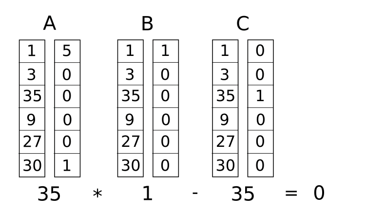
\[s \cdot a = (1,3,35,9,27,30) \cdot (5,0,0,0,0,1) = 35\]
\[s \cdot b = (1,3,35,9,27,30) \cdot (1,0,0,0,0,0) = 1\]
\[s \cdot c = (1,3,35,9,27,30) \cdot (0,0,1,0,0,0) = 35\]
Hence
\[ s \cdot a * s \cdot b - s \cdot c = 35 * 1 - 35 = 0\]
But instead of having just one constraint, we are going to have many constraints: one for each logic gate. There is a standard way of converting a logic gate into a (a, b, c) triple depending on what the operation is (+, -, * or /) and whether the arguments are variables or numbers. The length of each vector is equal to the total number of variables in the system, including a dummy variable ~one at the first index representing the number 1, the input variables x, a dummy variable ~out representing the output, and then all of the intermediate variables (sym1 and sym2 above);
First, we’ll provide the variable mapping that we’ll use:'~one', 'x', '~out', 'sym1', 'y', 'sym2'
Now, we’ll give the (a, b, c) triple for the first gate:
1 | a = [0, 1, 0, 0, 0, 0] |
which is \(x*x -sym1 = 0\)
Now, let’s go on to the second gate:
1 | a = [0, 0, 0, 1, 0, 0] |
which is \(sym1 * x = y\)
Now, the third gate:
1 | a = [0, 1, 0, 0, 1, 0] |
which is \( (x+y) * \sim one = sym2\)
Finally, the fourth gate:
1 | a = [5, 0, 0, 0, 0, 1] |
which is \((5 + sym2) * \sim one = \sim out\)
And there we have our R1CS with four constraints. The witness is simply the assignment to all the variables, including input, output and internal variables:[1, 3, 35, 9, 27, 30]
The complete R1CS put together is:
1 | A |
R1CS to QAP
The next step is taking this R1CS and converting it into QAP form, which implements the exact same logic except using polynomials instead of dot products. We do this as follows. We go from four groups of three vectors of length six to six groups of three degree-3 polynomials, where evaluating the polynomials at each x coordinate represents one of the constraints. That is, if we evaluate the polynomials at x=1, then we get our first set of vectors, if we evaluate the polynomials at x=2, then we get our second set of vectors, and so on.
We can make this transformation using something called a Lagrange interpolation.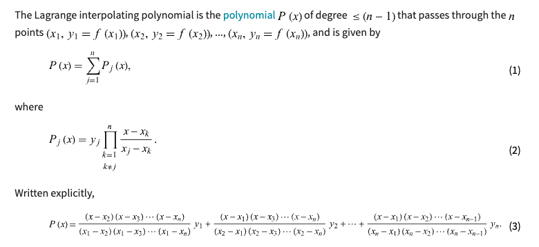
Now, let’s use Lagrange interpolation to transform our R1CS. What we are going to do is take the first value out of every a vector, use Lagrange interpolation to make a polynomial out of that (where evaluating the polynomial at i gets you the first value of the ith a vector), repeat the process for the first value of every b and c vector, and then repeat that process for the second values, the third, values, and so on. For convenience I’ll provide the answers right now:
Note: the intuition here is to think the R1CS A,B,C matrix vertically (column). For example, for the first column of A, the polynomial should pass (1,0), (2,0), (3,0), (4,5); the second polynomial shoudd pass (1,1), (2,0), (3,1), (4,)
1 | A polynomials |
Coefficients are in ascending order, so the first polynomial above is actually \(0.833 x^3 — 5 x^2 + 9.166 x - 5\)
Let’s try evaluating all of these polynomials at x=1.
1 | A results at x=1 |
Checking the QAP
Now what’s the point of this crazy transformation? The answer is that instead of checking the constraints in the R1CS individually, we can now check all of the constraints at the same time by doing the dot product check on the polynomials.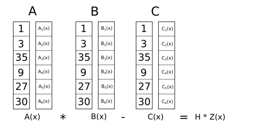
Because in this case the dot product check is a series of additions and multiplications of polynomials, the result is itself going to be a polynomial. If the resulting polynomial, evaluated at every x coordinate that we used above to represent a logic gate, is equal to zero, then that means that all of the checks pass; if the resulting polynomial evaluated at at least one of the x coordinate representing a logic gate gives a nonzero value, then that means that the values going into and out of that logic gate are inconsistent
To check correctness, we don’t actually evaluate the polynomial t = A . s * B . s - C . s at every point corresponding to a gate; instead, we divide t by another polynomial, Z, and check that Z evenly divides t - that is, the division t / Z leaves no remainder.
Z is defined as (x - 1) * (x - 2) * (x - 3) ... - the simplest polynomial that is equal to zero at all points that correspond to logic gates. It is an elementary fact of algebra that any polynomial that is equal to zero at all of these points has to be a multiple of this minimal polynomial, and if a polynomial is a multiple of Z then its evaluation at any of those points will be zero;
Note that the above is a simplification; “in the real world”, the addition, multiplication, subtraction and division will happen not with regular numbers, but rather with finite field elements — a spooky kind of arithmetic which is self-consistent, so all the algebraic laws we know and love still hold true, but where all answers are elements of some finite-sized set
KEA (Knowledge of Exponent Assumption)
Let \(q\) be a prime such that \(2q+1\) is also prime, and let \(g\) be a generator
of the order \(q\) subgroup of \(Z_{2q+1}^{\ast}\). Suppose we are given input \(q, g, g^a\) and want to output a pair \((C, Y )\) such that \(Y = C^a\). One way to do this is to pick some \(c \in Z_{q}\), let \(C = g^c\), and let \(Y = (g^a)^c\). Intuitively, `KEA1`` can be viewed as saying that this is the ‘only’ way to produce such a pair. The assumption captures this by saying that any adversary outputting such a pair must “know” an exponent \(c\) such that \(g^c = C\). The formalization asks that there be an “extractor” that can return \(c\). Roughly:
KEA1
For any adversary \(A\) that takes input \(q, g,g^a\) and returns \((C,Y)\) with \(Y = C^a\), there exists an ‘extractor’ \(\bar{A}\), which given the same inputs as \(A\) returns \(c\) such that \(g^c = C\)