introduction
Pairings allow you to check certain kinds of more complicated equations on elliptic curve points — for example, if \(P = G * p\), \(Q = G * q\) and \(R = G * r\), you can check whether or not \(p * q = r\), having just P, Q and R as inputs. This might seem like the fundamental security guarantees of elliptic curves are being broken, as information about p is leaking from just knowing P, but it turns out that the leakage is highly contained — specifically, the decisional Diffie Hellman problem is easy, but the computational Diffie Hellman problem (knowing P and Q in the above example, computing R = G * p * q) and the discrete logarithm problem (recovering p from P) remain computationally infeasible.
whereas traditional elliptic curve math lets you check linear constraints on the numbers (eg. if P = G * p, Q = G * q and R = G * r, checking 5 * P + 7 * Q = 11 * R is really checking that 5 * p + 7 * q = 11 * r), pairings let you check quadratic constraints (eg. checking e(P, Q) * e(G, G * 5) = 1 is really checking that p * q + 5 = 0).
Now, what is this funny e(P, Q) operator that we introduced above? This is the pairing. Mathematicians also sometimes call it a bilinear map; the word “bilinear” here basically means that it satisfies the constraints:
\[ e(P, Q + R) = e(P, Q) * e(P, R) \]
\[ e(P + S, Q) = e(P, Q) * e(S, Q) \]
Note that + and * can be arbitrary operators; when you’re creating fancy new kinds of mathematical objects, abstract algebra doesn’t care how + and * are defined, as long as they are consistent in the usual ways.
If P, Q, R and S were simple numbers, then making a simple pairing is easy: we can do e(x, y) = 2^xy. Then, we can see:
\[e(3, 4+ 5) = 2^(3 * 9) = 2^{27}\]
\[e(3, 4) * e(3, 5) = 2^(3 * 4) * 2^(3 * 5) = 2^{12} * 2^{15} = 2^{27} \]
However, such simple pairings are not suitable for cryptography because the objects that they work on are simple integers and are too easy to analyze;
It turns out that it is possible to make a bilinear map over elliptic curve points — that is, come up with a function e(P, Q) where the inputs P and Q are elliptic curve points, and where the output is what’s called an \(F_{p^¹²}\) (extension field) element
An elliptic curve pairing is a map G2 x G1 -> Gt, where:
- G1 is an elliptic curve, where points satisfy an equation of the form y² = x³ + b, and where both coordinates are elements of F_p (ie. they are simple numbers, except arithmetic is all done modulo some prime number)
- G2 is an elliptic curve, where points satisfy the same equation as G1, except where the coordinates are elements of \(F_{p^¹²}\). we define a new “magic number” w, which is defined by a 12th degree polynomial like w^12 - 18 * w^6 + 82 = 0
- Gt is the type of object that the result of the elliptic curve goes into. In the curves that we look at, Gt is \(F_{p^¹²}\)
The main property that it must satisfy is bilinearity, which in presented above
There are two other important criteria:
- Efficient computability (eg. we can make an easy pairing by simply taking the discrete logarithms of all points and multiplying them together, but this is as computationally hard as breaking elliptic curve cryptography in the first place, so it doesn’t count)
- Non-degeneracy (sure, you could just define e(P, Q) = 1, but that’s not a particularly useful pairing)
math intuition behind paring
The math behind why pairing functions work is quite tricky and involves quite a bit of advanced algebra going even beyond what we’ve seen so far, but I’ll provide an outline. First of all, we need to define the concept of a divisor, basically an alternative way of representing functions on elliptic curve points. A divisor of a function basically counts the zeroes and the infinities of the function. To see what this means, let’s go through a few examples. Let us fix some point P = (P_x, P_y), and consider the following function:
\[f(x, y) = x - P_x\]
The divisor is [P] + [-P] - 2 * [O] (the square brackets are used to represent the fact that we are referring to the presence of the point P in the set of zeroes and infinities of the function, not the point P itself; [P] + [Q] is not the same thing as [P + Q]). The reasoning is as follows:
- The function is equal to zero at P, since x is P_x, so x - P_x = 0
- The function is equal to zero at -P, since -P and P share the same x coordinate
- The function goes to infinity as x goes to infinity, so we say the function is equal to infinity at O. There’s a technical reason why this infinity needs to be counted twice, so O gets added with a “multiplicity” of -2 (negative because it’s an infinity and not a zero, two because of this double counting).
The technical reason is roughly this: because the equation of the curve is x³ = y² + b, y goes to infinity “1.5 times faster” than x does in order for y² to keep up with x³; hence, if a linear function includes only x then it is represented as an infinity of multiplicity 2, but if it includes y then it is represented as an infinity of multiplicity 3.
Where a, b and c are carefully chosen so that the line passes through points P and Q. Because of how elliptic curve addition works (see the diagram at the top), this also means that it passes through -P-Q. And it goes up to infinity dependent on both x and y, so the divisor becomes [P]+ [Q] + [-P-Q] - 3 * [O]. (multiplicity of 3 because it involves y)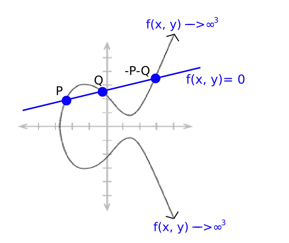
We know that every “rational function” (ie. a function defined only using a finite number of +, -, * and / operations on the coordinates of the point) uniquely corresponds to some divisor, up to multiplication by a constant (ie. if two functions F and G have the same divisor, then F = G * k for some constant k).
For any two functions F and G, the divisor of F * G is equal to the divisor of F plus the divisor of G (in math textbooks, you’ll see (F * G) = (F) + (G)), so for example if f(x, y) = P_x - x, then (f³) = 3 * [P] + 3 * [-P] - 6 * [O]; P and -P are “triple-counted” to account for the fact that f³ approaches 0 at those points “three times as quickly” in a certain mathematical sense.
Note that there is a theorem that states that if you “remove the square brackets” from a divisor of a function, the points must add up to O ([P] + [Q] + [-P-Q] - 3 * [O] clearly fits, as P + Q - P - Q - 3 * O = O), and any divisor that has this property is the divisor of a function.
Tate pairings
Consider the following functions, defined via their divisors:
- (F_P) = n * [P] - n * [O], where n is the order of G1, ie. n * P = O for any P
- (F_Q) = n * [Q] - n * [O]
- (g) = [P + Q] - [P] - [Q] + [O]
Now, let’s look at the product F_P * F_Q * g^n. The divisor is:
n * [P] - n * [O] + n * [Q] - n * [O] + n * [P + Q] - n * [P] - n * [Q] + n * [O]
Which simplifies neatly to:
n * [P + Q] - n * [O]
Notice that this divisor is of exactly the same format as the divisor for F_P and F_Q above. Hence, F_P * F_Q * g^n = F_(P + Q).
Now, we introduce a procedure called the “final exponentiation” step, where we take the result of our functions above (F_P, F_Q, etc.) and raise it to the power z = (p¹² - 1) / n, where p¹² - 1 is the order of the multiplicative group in F_p¹² (ie. for any x ϵ F_p¹², x^(p¹² - 1) = 1). Notice that if you apply this exponentiation to any result that has already been raised to the power of n, you get an exponentiation to the power of p¹² - 1, so the result turns into 1. Hence, after final exponentiation, g^n cancels out and we get F_P^z * F_Q^z = F_(P + Q)^z. There’s some bilinearity for you.
Now, if you want to make a function that’s bilinear in both arguments, you need to go into spookier math, where instead of taking F_P of a value directly, you take F_P of a divisor, and that’s where the full “Tate pairing” comes from. To prove some more results you have to deal with notions like “linear equivalence” and “Weil reciprocity”, and the rabbit hole goes on from there. You can find more reading material on all of this [2] and he[3].
Every elliptic curve has a value called an embedding degree; essentially, the smallest k such that p^k - 1 is a multiple of n (where p is the prime used for the field and n is the curve order). In the fields above, k = 12, and in the fields used for traditional ECC (ie. where we don’t care about pairings), the embedding degree is often extremely large, to the point that pairings are computationally infeasible to compute; however, if we are not careful then we can generate fields where k = 4 or even 1.